David A. Kenny
September 4, 2012
Being
revised after 8 years.
Please send suggestions and corrections.
Estimation with Instrumental Variables
One way of
identifying models that cannot be estimated by using multiple
regression is through the use of instrumental variables. For multiple
regression to be used, the endogenous variable’s disturbance must be
uncorrelated with each of the causal variables. There are three reasons
why such a correlation might exist:
- Spuriousness (third or omitted variable): A
variable causes both the endogenous
variable and one of its causal variables and that variable is not
included in the model.
- Reverse Causation (feedback Model): The endogenous
variable causes, either directly or indirectly, one of its causes.
- Measurement
Error: There is measurement error in a causal variable.
Given one of the
above, one or more causal variable is correlated with the disturbance
of the endogenous
variable. Thus, multiple regression cannot be used to estimate the
causal coefficients. However, for each of these cases, estimation using one or more instrumental
variable can be used to identify the model.
What Is an Instrumental Variable?
Denote Y as the endogenous variable, U as its disturbance, X as the variable correlated with U and causing Y, I as an instrumental variable, and Z as a variable that causes X and Y but not needing an instrumental variable. The identifying feature of an instrumental variable is that I is assumed not to directly cause Y: The path from I to Y is fixed zero. The zero path is given by theory, not by statistical analysis. That is, do not regress Y on X, I, and Z, and select I by seeing which variables have coefficients that are not significantly different from zero. Conditions for estimation using instrumental variables:
1) The variable I must not directly cause Y or
be correlated with U.
2) For a given structural equation, there must be as many or more I
variables as there are variables needing an instrument.
3) The variable I must cause the variable that needs an instrument.
(For
more details of the identification of models with instrumental variables.)
Consider
first the use of an instrumental variable with an omitted variable as in the
figure below:
‑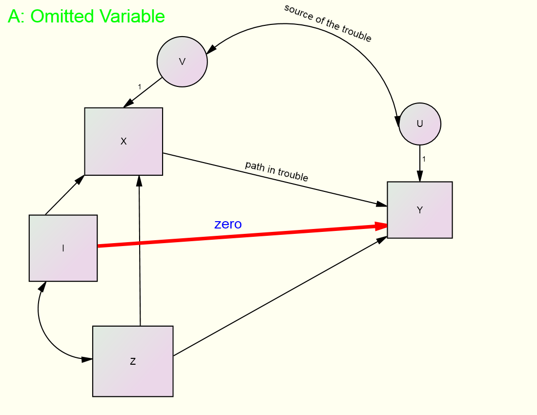
In the
figure, the goal is to estimate the effect of X and Z on Y, but there is a
problem. The variable X is correlated
with U, the disturbance in Y. That
correlation is due to the fact that a variable not included in the model (the
omitted variable) causes both X and Y which makes the disturbances of X and Y
correlated. So the path from X to Y is
“in trouble.” However, there is an
instrumental variable, variable I in the figure, which does not cause Y (the
red zero path) and is not correlated with U.
Note too it must be assumed that the source of the covariation between I
and X is a causal effect from I to X. If
X caused I, then I would be correlated with U which would be problematic.
Next
consider the use of instrumental variables in a feedback model as in the figure
below:
‑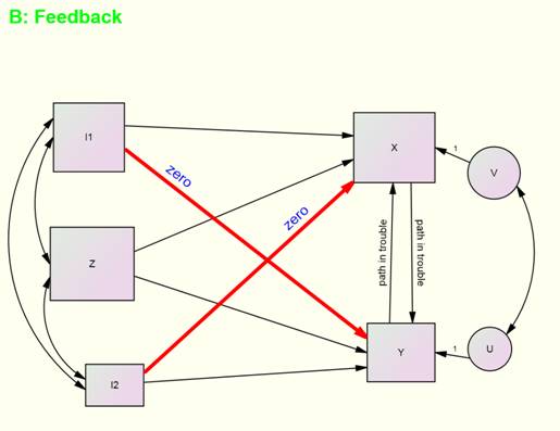
In the
figure, the goal is to estimate the effect of X and Z on Y and the effect of Y
and Z on X, but there is a problem. The
variable X is correlated with U, the disturbance in Y, and also the variable Y
is correlated with V, the disturbance in X.
That correlation is due to the feedback loop between X and Y, as well as
the correlation between their disturbances.
Both the path from X to Y and Y to X are “in trouble” and each needs a
different instrumental variable. Luckily,
there are two instrumental variables, I1 and I2. Consider the effect of Y equation. Because I1 does not cause Y (the
red zero path) and is not correlated with U, the variable I1 can be
used as an instrumental variable. Also,
because I2 does not cause X (the other red zero path) and is not
correlated with V, the variable I2 can be used as an instrumental
variable. Notice that for the model to
be empirically identified, I1 must cause X, and I2 must
cause Y, i.e., these two paths cannot be small.
Lastly
consider the use of instrumental variables with measurement error in a causal
variable, as in the following figure:
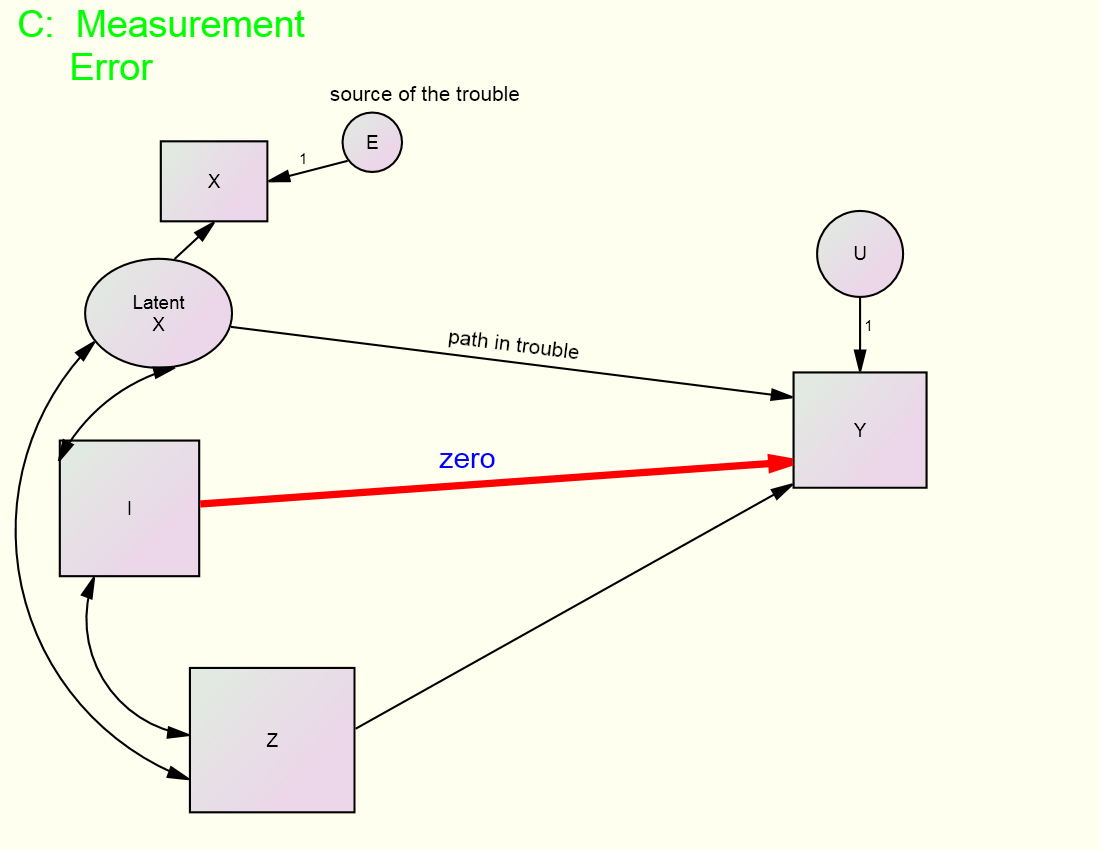
A multiple
indicator strategy (see CFA webpage) is much more commonly used to identify models with
measurement error but estimation using instrumental variable can also be used. In the figure, the goal is to estimate the
effects of X, actually latent X, and Z on Y, but there is a problem. The variable X has measurement error. So the path from X to Y is “in trouble” and
the source of that trouble in the presence of measurement error in X. There is an instrumental variable, variable I
in the figure, which does not cause Y (the red zero path) and is not correlated
with U to identify the model.
Instrumental variable estimation can be used to estimate the parameters
of this model. Notice too that if latent
X had two indicators with correlated, the model would still be identified.
Finding an Instrumental Variable
It is not always an easy task to locate an instrumental variable. One thing not to do is to try to locate one empirically. That is, you should not locate an instrumental variable by running a regression, seeing which path is zero, and using that causal variable as an instrument. The problem with this approach is that coefficients are biased because multiple regression cannot be used to estimate the coefficients from this equation.There are four related
strategies for finding instrumental variables:
different data source, mediation, longitudinal data, and compliance
modeling.
Different data source: Consider the study by Duncan,
Haller, and Portes (1968) which is a feedback model in which an adolescent’s
educational aspirations causes his or her friend’s and vice versa. As instrumental variables, Duncan et al.
(1968) used each child’s family background (e.g., parental socio-economic
status) as instrumental variables. The
assumption made is that parental background affects the child’s own educational
aspirations, but not the child’s peer’s educational aspirations. The two sets of instrumental variables come
from two different data sources: the child and the peer. Also see Sadler and Woody (2003) for another
dyadic example and Heath,
Neale, Hewitt, Eaves, Kessler, and Kendler (1993) for an example with families.
Mediation: If it is known that the effect of
X on Y is mediated by M, the variable X can be used as instrumental variable to
estimate the M to Y effect. See for
instance, Felson (1981) used symbolic interactionism which posits that
perceptions of significant others are mediated by reflected appraisals to
affect self-concept. He used perceptions
of significant others as the instrumental variable to allow for a feedback model
between reflected appraisals and self-concept.
Longitudinal data: Consider three-wave data where X1
(the subscript denotes time) causes X2 which in turn causes X3,
a model commonly called a first order autoregressive model. The path from X2 to X3
is identified even allowing for measurement error in X2 by using X1
as an instrumental variable. This
strategy is discussed later when autoregressive
models are presented later in this tutorial. Note that X1 may have measurement
error but that is not problematic in this case.
Compliance modeling: There is an intervention, called
Treatment, to which units are randomly assigned. Some people comply with treatment and some do
not and this variable is called Compliance.
It is assumed that the effect of Treatment on Outcome works through
Compliance, but the disturbance in Compliance may be correlated with Outcome. Treatment can be used as an instrumental
variable to estimate the effect of Compliance on the outcome. Note that the indirect effect of Treatment on
Outcome is the “intention to treat” effect.
To learn more consult Greenland (2000). Note too that this strategy can be used when
there is a manipulated variable and a manipulation check variable that
operationalizes how it is the manipulation affects the outcome variable.
Identification Issues
Empirically Underidentified Models
Some models with instrumental variable have empirical under-identification
issues. For instance Model A with
Omitted Variables, if the path from I to X is weak, the model will be
empirically under-identified. For Model B with Feedback, to identify the path
from X to Y, the I1 to X path cannot be weak, and to identify the
path from Y to X, the I2 to Y path cannot be weak. Finally for model C with measurement error
the partial correlation between I1 and X controlling for Z cannot be
weak. If these paths or correlations are
weak, the estimates might well be wild and the standard errors large.
Over-identified Models
So far it has been assumed that for each “variable in trouble” there is one
instrumental variable. In some cases,
there is an excess of instrumental variables.
For instance in Duncan et al. (1968) there are three measures of
parental background. Thus, there are an
excess of two instruments for each equation and because there are two
equations, the model degrees of freedom is four.
If a given structural
equation is over-identified because there are two or more instrumental
variables, a test can be made that both zero paths assumption. The problem is that if the null hypothesis of
zero paths is rejected, it is not clear which of the zero paths are non-zero. If fact it is possible that both are
non-zero. (Note also that even if the
model with multiple zero paths has good fit, it may still be the case that all
of the paths are biased in the same direction, and the assumption of zero paths
is invalid. However, if there are three
or more paths and only one is non-zero, it can be determined when fit is
improved by freeing up one path.
Estimation of Models with Instrumental Variables
Most models with instrumental variables are currently usually estimated using an SEM program using maximum likelihood. Briefly discussed here are two alternative methods of estimation.
Use of
Instrumental Variable Estimation Instead of Maximum Likelihood
Ken Bollen (1996) has suggested using instrumental variable estimation as an
alternative to the standard maximum likelihood estimation. One major advantage of this approach is that
estimates are less sensitive to miss-specifications that occur elsewhere in the
model. Moreover, this approach can test
the over-identifying restrictions for each parameter in the model. Unfortunately, no SEM package currently
offers instrumental variable estimation as an alternative.
Two-Stage Least Squares (2SLS)
An old- fashioned way to
estimate such models is 2SLS, which is now described. Even though this method is not used very
often these days, by understanding 2SLS, a better understanding of how models
with instrumental variables are estimated can be obtained.
Although this method is not
currently used very often for the estimation of models with instrumental
variables, it is instructive to understand how it works.
- Stage 1: Regress each variable needing an instrument on
the set of I and Z variables. To avoid empirical
under-identification, the coefficient for I should be non-trivial. Using
the coefficients from this stage, compute predicted X variables.
- Stage 2: Regress Y on the stage 1 predicted variables
and the set of Z variables.
In actuality,
2SLS computer programs execute the two steps in a single stage or step.
2SLS Example
The structural equation for models A and C above is as follows:
Y = aX + bZ + U
where X is correlated with
U. For this example, variable I serves as an instrumental variable for X
in the Y equation and it must be assumed that the effect of I on Y controlling
for X and Z is zero and that I and Z are uncorrelated with U.
For the Y equation:
Stage 1: Regress X on I and Z.
Stage 2: Regress Y on Z and the stage 1 predicted score for X. The effect of the predicted X score provides
an estimate of path a.
As a second example,
consider the two structural equations for the feedback model B above:
Y = aX + bZ + cI2 + U
X = dY + eZ + fI1 + V
For the X equation:
Stage 1: Regress X on I1 and Z.
Stage 2: Regress Y on Z, I2, and the stage 1 predicted
score for X. The effect of the predicted
X score provides an estimate of path a.
For
the X equation:
Stage 1: Regress Y on I2 and Z.
Stage 2: Regress X on Z, I1, and the stage 1 predicted
score for Y. The effect of the predicted
Y score provides an estimate of path d.
See Johnston and DiNardo
(1997) for more details about two-stage least squares and other methods of
estimation for models with instrumental variables.
References
Bollen, K. A. (1996). An alternative two stage least squares (2SLS)
estimator for latent variable equations.
Psychometrika, 6, 109-121.
Duncan, O. D., Haller, H. O., & Portes, A. (1968). Peer influences on aspirations: A reinterpretation. American Journal of Sociology, 74, 119–137
Felson, R. B.
(1981). Self- and reflected appraisal among
football players: A Test of the Meadian hypothesis. Social Psychology Quarterly. 44, 116-126.
Heath, A.C., Neale, M.C., Hewitt, J.K.,
Eaves, L.J., Kessler, R.C., & Kendler, K. S. (1993). Testing hypotheses
about direction of causation using cross-sectional family data. Behavior Genetics, 23, 29-50.
Johnston, J., &
DiNardo, J. (1997). Econometric methods,
4th ed. New York: McGraw Hill.
Sadler, P., & Woody, E. (2003). Is who you are who you’re talking to? Interpersonal style and complementarity in mixed-sex interactions. Journal of Personality and Social Psychology, 84, 80-96.