David A. Kenny
September 15, 2018
Moderator Variables: Introduction
Categorical Moderator and Causal Variables
Categorical Moderator and a Continuous
Causal Variable
Continuous Moderator and a
Categorical Causal Variable
Continuous Moderator and Causal
Variable
Other Issues
Bibliography
Moderator Variables: Introduction
Basic DefinitionsWe begin with a linear causal relationship in which the variable X is presumed to cause the variable Y. A moderator variable M is a variable that alters the strength of the causal relationship. So for instance, psychotherapy may reduce depression more for men than for women, and so we would say that gender (M) moderates the causal effect of psychotherapy (X) on depression (Y). Most moderator analysis measure the causal relationship between X and Y by using a regression coefficient. Although classically, moderation implies a weakening of a causal effect, a moderator can amplify or even reverse that effect. Complete moderation would occur in the case in which the causal effect of X on Y would go to zero when M took on a particular value. The reader might consult papers by Kraemer and colleagues (2001; 2002) for a related but somewhat different approach to defining and testing of moderators. Frazier, Tix, and Barron (2004) provide a very good introduction to the topic of moderation and Marsh, Hau, Wen, Nagengast, and Morin. (2011) for a more detailed discussion of the topic. A moderation analysis is an exercise of external validity in that the question is how universal is the causal effect.
A key part of moderation is the measurement of X to Y causal relationship for different values of M. We refer to the effect of X on Y for a given value of M as the simple effect X on Y.
Deciding which variable is the moderator depends in large part on the researcher's interest. For the earlier example in which gender moderates the effect of psychotherapy, if one was a gender researcher, one might say that psychotherapy moderates the effect of gender.
Causal Assumptions
If X is a randomized variable, there is no causal ambiguity. Uncertainties arise when X is not randomized. If X is not manipulated, then the direction of causation must be assumed based on
theory or common sense. As shown in Judd and Kenny (2010), it is even possible
that the moderator effect can reverse if the direction of causation is flipped
(presuming that Y causes X instead of vice versa).
In a moderator analysis, if X is not manipulated, the researcher
needs to justify the choice of causal direction.
Timing of Measurement
Ideally the moderator should be
measured prior to variable X being
measured. So if X is manipulated,
then M should be measured prior to X being manipulated. Of course, if M is a variable that does not change
(e.g., race), the timing of its measurement is less problematic.
It is possible, but quite complicated, but M can be both a mediator and a
moderator (see Kraemer et al. (2001) for a different point of view.
Moderator and Causal Variable
Relationship
If X is a manipulated variable, in principal, there should be no
relationship between X and M. If X is not randomized, it
might be correlated with M. Unlike
mediation, there is no need for X and M to be correlated and that
correlation has no special interpretation. However, if X and M are too highly
correlated, there can be collinearity issues in XM being too highly correlated with X and M.
Measurement of Moderation
Generally, moderator effects are
indicated by the interaction of X and M in explaining Y. The following multiple regression
equation is estimated:
Y = i + aX + bM + cXM + E (1)
The interaction of X and M or coefficient c measures the moderation effect. Note that path a measures the simple effect of X, sometimes called the main effect of X, when M equals zero. As will be seen, the test of moderation is not always operationalized by the product term XM. Given Equation 1, the effect of X on Y is a + cM. Thus, the effect of X on Y depends on the value of M. It is noted that the effect of X on Y equals zero when M equals –a/c, which may or may not be a plausible value of M.
Alternative Interpretations of Moderator
Effects
Finding
that c is statistically significant
does not prove moderator effects. One
major worry is non-additivity. Consider
the case in which the relationship between X and Y is nonlinear. For instance, X is income and Y is
work motivation. Imagine that the
relationship between the two is nonlinear such that if X is small the relationship is larger than when X is large. If age were tested as a moderator the
income-motivation relationship, then because younger workers make less money,
we would find the “moderator” effect, that the income-motivation relationship
is stronger for younger than for older workers.
Another worry is the actual moderator may not be the moderator but some other variable with which the moderator correlates. For instance, if we find that gender is a moderator, the real moderator might be height, masculinity-femininity, expectations of others, or income. Unless the moderator is a manipulated variable, we do not know whether it is a “true” moderator or just a “proxy” moderator.
Level of Measurement of the Variables
It is
presumed here and throughout that the outcome variable is measured at the
interval level of measurement. Should
the outcome be a dichotomy, logistic regression would need to be used (Hayes & Matthes, 2009).
The remainder of the page is organized around the levels of measurement of the moderator and the causal variable. The causal variable, X, can either be categorical (typically a dichotomy) or a continuous variable. So for instance, X might be psychotherapy versus no psychotherapy (a dichotomy) or it might be the amount of psychotherapy (none, one month, two months, or six months; a continuous variable). Much in the same way, the moderator or M can be either categorical (e.g., gender) or continuous (e.g., age). Readers are encouraged to read the next two sections, even if they are more interested in one of the other cases, as many key concepts in mediation are discussed there.
Categorical Moderator and Causal Variables
When both X and M are dichotomous (i.e., each have two levels), we have a 2 x 2 design. So for instance, psychotherapy (therapy versus no therapy), might be more effective for women than for men. We denote the four cells as X1M1, X1M2, X2M1,and X2M2. To estimate the above regression equation, we need to dummy code the moderator and the causal variable. So for instance, if we use codes of zero and one, then we have the following interpretations of the coefficients in the above multiple regression equation (Equation 1):
a – the effect of X when M is zero (the simple effect of X when M is zero)
b – the effect of M when X is zero
c – how much the effect of X changes as M goes from 0 to 1
The focus on c because it captures the moderator effect. If c is positive, then it indicates that the effect of X on Y increases as M goes from 0 to 1. If c is negative, then it indicates that the effect of X on Y decreases as M goes from 0 to 1. Obviously the interpretation of moderator depends very much on how X and M are coded.
If effect coding (one value of X and M is 1 and the other value is –1) is used, the interpretation of the coefficients is as follows:
a – the effect of X averaged across M (i.e., when M = 0)
b – the effect of M averaged across X (i.e., when X = 0)
c – half of how much the effect of X changes as M goes from -1 to 1
Which particular coding method that is used is largely a matter of personal preference. The important thing is to know what coding system is used and interpret coefficients accordingly. Although coding affects the coefficients, it does not affect the inferential statistic for the test of the interaction (but it does affect the tests of main effects), the multiple correlation, the predicted values, and the residuals. It is generally inadvisable to trim out of the multiple regression equation the main effects if the interaction is present in the equation.
Regardless which coding system is used, there are four means because the design is 2 x 2. If effect coding were used, the means would equal (where i is the intercept in the regression equation):
Cell Coding Predicted Mean
X1M1 X = -1; M = -1 i – a – b + c
X2M1 X = 1; M = -1 i + a – b – c
X1M2 X = -1; M = 1 i – a + b – c
X2M2 X = 1; M = 1 i + a + b + c
There might be an interest in the effect of the causal variable or X for each of the levels of the moderator or the simple effects of X. To estimate the simple effects, a different regression equation is run and in each we recode the moderator so that a given level is set to zero (Aiken & West, 1991). If we want to test the effect of X when the M = 1, the equation is run but M is not used but M׳ = M – 1. Coefficient b is now the simple effect of X on Y when M is 1, because when M = 1, M׳is zero.
If X or M have more than two levels, then multiple dummy variables are needed (the number of levels less one), and moderation is tested by a set of product variables.
If there are covariates (variables that cause Y and measured prior to Y), they can be entered into the equation. If the covariates are themselves considered to be moderators, then they would be allowed to interact with X. Note that predicted values for the four cells would no longer exactly equal the mean for the cell and so they should be referred to as least squares means.
Effect Size Measurement of Moderator
Effects and Power Analysis
One
can use traditional measures of effect size in measuring moderator effects f2 (see below). However, what seems preferable is to use a d change where d is Cohen's d – mean
difference divided by pooled standard deviation. That is, we measure the d for each of
the two levels of M and compare
them. In computing the two d’s, we should use the same standard
deviation. For instance, we might
state: The effect of psychotherapy on
depression yields a d of 0.4 for men
and a d of 0.7 for women or
0.3. Because both M and X are dichotomies,
this d change measure is itself a d. Because the design is 2 X 2, the estimate of
the moderator effects can be viewed as a difference between two means (X1M1 and X2M2 vs. X2M1 and X1M2). Using these two means a d can be computed and a power analysis
can be undertaken.
Categorical Moderator and Continuous Causal Variable
An example of this case, M is race, X is a personnel test, and Y is some job performance score. Generally, it is assumed that the effect of X on Y is linear. It is also assumed (but it can be tested, see below) that the moderation is linear. That is, as M varies, the linear effect of X on Y might vary. Thus, the linear relationship increases or decreases as M increases.
It is almost always preferable to measure the linear effect by using a regression coefficient and not a correlation coefficient.
More Complex Specification
Nonlinear
moderation refers to effect of X changing as function of M, but that
change is nonlinear. The typical way to estimate nonlinear moderation would be
to estimate the following equation:
Y = d + a1X + b1M + b2M2 + c1XM + c2XM2 + E (2)
Nonlinear moderation can be tested by determining if c2 is different from zero. (Note that M2 effects can only be estimated if M takes on at least 3 values.) The effect of X in Equation 2 is a1 + (c1 + c2M)M which would be interpreted as follows:
If c1 were positive and c2 positive, then the effect of X on Y would be increasing as M increases, and this increase is increasing as M increases, accelerating.
If c1 were positive and c2 negative, then the effect of X on Y would be increasing as M increases, but this increase is declining as M increases, de-accelerating.
If c1 were negative and c2 positive, then the effect of X on Y would be decreasing as M increases, but this decrease is declining as M increases, de-accelerating.
If c1 were negative and c2 negative, then the effect of X on Y would be decreasing as M increases, but this decrease is increasing as M increases, accelerating.
Baron and Kenny (1986, page 1175) discuss alternative specifications of moderation. For instance, the moderator might act as a threshold variable and there would be no effect of the causal variable when the moderator is low, but at a certain value of the moderator the effect emerges. In this case, the moderator is no longer continuous, but rather it is dichotomized at the point of the threshold. The difficulty is that threshold point must be known a priori and cannot be obtained by a simple median split. [The value of M at which the effect of X on Y changes might be empirically determined by adapting an approach described by Hamaker, Grasman, and Kamphuis (2010)].
Effect Size and Power
The most common measure of
effect size in tests of moderation is f2 (Aiken & West, 2001) which equals the unique variance explained by the
interaction term divided by sum of the error and interaction variances. When X and M are dichotomies f2 equals the d2/4 where d is the d difference measure described above. Cohen (1988) has suggested that f2 effect sizes of 0.02,
0.15, and 0.35 are termed small, medium, and large,
respectively. However, Aguinis, Beaty,
Boik, and Pierce (2005) has shown that the
average effect size in tests of moderation is only 0.009. Perhaps a more realistic standard for effect
sizes might be 0.005, 0.01, and 0.025 for small, medium,
and large, respectively. We note
that even these values are "optimistic" given the Aguinis et al.
(2005) review.
If f2 is known, one can conduct a power analysis using a power analysis program. For instance, if f2 is assumed to be 0.025, one needs a sample size of 316 to have 80 percent power. Power for tests of moderation is very low when one or both of the variables are continuous (McClelland & Judd, 1993). Likely, the much greater interest in mediation over moderation is due to the low power in tests of moderation.
Simple Effects
There are three methods to
determine simple effects. The first method is to estimate the simple effects
using the regression equation. Using Equation 1, we solve for a + cM. For instance, if the moderation regression equation were 5 + 2X + 3M + 1XM and we wanted to
estimate the effect of X when M is 2, that effect would be 2 + (1)(2)
or 4.
The second method is to re-estimate separate regression equation but transform M by subtracting 2 or M' = M – 2. For this new equation, the effect of X refers to the case in which M is 2. This second method should result in the same answer as the first.
The third method requires that M take on a few values. Separate regression equations would be estimated for each value of M. This method does not assume homogeneity of error variances and so it would likely produce estimates different from the previous two.
Continuous Moderator and Categorical Causal Variable
An example is that the socioeconomic status moderates the effect of some intervention. One key issue is to center the variable of socioeconomic status; i.e., make sure that zero is a meaningful value for the moderator.
We may want to determine the effect of X for various levels of the moderator, M, i.e., simple effects. In principal, the values of M would be chosen using some sort conceptual rationale. For instance, if IQ were the moderator, we might use 140 (genius level) and 100 (average level) to compute the effects of X on Y. More commonly, the values are one standard deviation above the mean of M and one standard deviation below the mean of M. To obtain these estimates we use either the first or second method described above.
Continuous Moderator and Causal Variable
One key question is the assumption of how the moderator changes the causal relationship between X and Y. Normally, the assumption is made that the change is linear: As M goes up or down by a fixed amount, the effect of X on Y changes by a constant amount. Alternatively, M may have a different type of effect: Threshold – The effect of X on Y changes when M is greater than a certain value; Discrepancy – When X and M are measured using the same units, the absolute difference between X and M is what matters (see also Edwards, 1995). The key point is that moderation is not always best captured by a product term.
If a product term is used, one must assume that both X and M are measured without error, an often dubious assumption. Latent variables are discussed below.
Centering of both X and M is necessary if neither have zero as a meaningful value. To interpret the results and determine simple effects, the effect of X at various levels of M would be measured. Ideally, the levels of M would be theoretically motivated. If not possible, one might use M at the mean and at plus and minus one standard deviation from the mean.
Power of tests of moderation with two continuous variables is particularly low (McClelland & Judd, 1993).
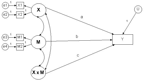
Latent Variables
In this case one latent variable interacts with another latent
variable. This is the most complicated case. Kenny and Judd (1984)
have developed a solution using product indicators of X1M1, X1M2, X2M1,
and X2M2, but
it is quite complicated with many nonlinear constraints and it requires a large
sample size to have sufficient power and the assumption of normality to
identify the model. Klein and Moosbrugger (2000) have developed a method
of estimation that does not require nonlinear constraints and their procedure
is described by Marsh, Wen, and Hau (2004). This method uses “paired” product indicators (X1 with M1 and X2 with M2).
Three additional issues that are discussed here briefly are repeated measures, multilevel modeling, meta-analysis, moderated mediation or mediated moderation, and mixture modeling.
Repeated Measures
All of the above
discussion presumes that the design is between participants. In some cases, the
design is repeated measures. Judd, Kenny, and McClelland (2001)
describe moderator analyses in this case. In essence, moderation is indicated
by computing a difference score across conditions and determining whether the
moderator predicts that difference: Because the difference score measures the
effect of X on Y for each person, using it as the outcome variable gives an
ideographic measure the causal effect and it is then determined if the
moderator predicts that causal effect. Moderation with repeated measures can also be handled by multilevel
modeling.
Multilevel Modeling
In some situations
the data are said to be clustered,
and a multilevel model is needed to model the nonindependence due to
clustering. For instance, there might be
students in classrooms with students being a level 1 and classrooms at level 2.
Sometimes, there are level 1 moderators, these being moderators that vary
within the classroom. More typically there are level 2 moderators, these being
moderators that vary between classrooms. Note too that X can be at either level 1 or level 2.
If X is measured at level 1, one can determine a generic moderator, that is, measure the extent to which there is variation in the X-Y relationship. Evidence of generic moderation would be obtained if there was variation in the X-Y slopes.
Meta-analysis
Much of
meta-analysis involves the study of moderation. If a variable predicts effect sizes, that variable is moderator. Moreover, as with multilevel modeling, one
can test for a generic moderator by determining if effect sizes vary more than
would be expected by sampling error. One
of the key tasks in meta-analysis is the understanding or what are the
moderators of the effect.
Mediated Moderation and Moderated
Mediation
In mediated
moderation, the moderation disappears when the mediator is introduced. In moderated mediation, the pattern of
mediation varies as a function of the moderator. See my mediation page for more
information.
Papers by Muller, Judd, and Yzerbyt (2005) and Edwards and Lambert (2007) discuss the relationship between mediated moderation and moderated mediation. They also present examples of each.
Mixture Modeling
We can use mixture
modeling to search for a "latent" moderator. In such a case, we measure X and Y and then we allow for latent classes which would be a categorical moderating
variable.
Aguinis, H., Beaty, J. C., Boik, R. J., & Pierce, C. A. (2005). Effect size and power in assessing moderating effects of categorical variables using multiple regression: A 30-year review. Journal of Applied Psychology, 90, 94-107.
Aiken, L. S., & West, S. G. (1991). Multiple regression: Testing and interpreting
interactions.
Baron, R. M., & Kenny, D. A. (1986). The moderator-mediator variable distinction in social psychological research: Conceptual, strategic and statistical considerations. Journal of Personality and Social Psychology, 51, 1173-1182.
Cohen, J. (1988). Statistical power analysis for the behavioral sciences.
Edwards, J. R., & Lambert L. S. (2007). Methods for integrating moderation and mediation: A general analytical framework using moderated path analysis. Psychological Methods, 12, 1-22.
Frazier, P. A., Tix, A. P. & Barron, K. E. (2004). Testing moderator and mediator effects in counseling psychology research. Journal of Counseling Psychology, 51, 115-134.
Hamaker, E. L., Grasman, R. P. P. P., & Kamphuis, J.
H. (2010). Regime-switching models to study psychological processes. In P. C.
M. Molenaar & K. M. Newell (Eds.), Individual pathways of change:
Statistical models for analyzing learning and development, 155-168.
Hayes, A. F., & Matthes, J. (2009). Computational procedures for probing interactions in OLS and logistic regression: SPSS and SAS implementations. Behavior Research Methods, 41, 924-936.
Judd, C. M., & Kenny, D. A. (2010). Data analysis. In D. Gilbert, S. T. Fiske, G. Lindzey (Eds.), The handbook of social psychology(5th ed., Vol. 1, pp. 115-139), New York: Wiley.
Judd, C. M., Kenny, D. A., & McClelland, G. H. (2001). Estimating and testing mediation and moderation in within-participant designs. Psychological Methods, 6, 115-134.
Kenny, D. A., & Judd, C. M. (1984). Estimating the nonlinear and interactive effects of latent variables. Psychological Bulletin, 96, 201-210.
Klein, A. G., & Moosbrugger, H. (2000). Maximum likelihood estimation of latent interaction effects with the LMS method. Psychometrika, 65, 457-474.
Kraemer, H. C., Stice, E., Kazdin, A., Offord, D., & Kupfer, D. (2001). How do risk factors work together? Moderators, mediators, independent, overlapping, and proxy risk factors. American Journal of Psychiatry, 158, 848-856.
Kraemer H. C., Wilson G. T., Fairburn C. G., & Agras W. S. (2002). Mediators and moderators of treatment effects in randomized clinical trials. Archives of General Psychiatry, 59, 877-883.
Marsh, H. W., Hau, K. T., Wen, Z., Nagengast, B., & Morin, A. J. S. (2011). Moderation. In Little, T. D. (Ed.), Oxford handbook of quantitative methods. New York: Oxford University Press.
Marsh, H. W., Wen, Z. L., & Hau, K. T. (2004). Structural equation models of latent interactions: Evaluation of alternative estimation strategies and indicator construction. Psychological Methods, 9, 275-300.
McClelland, G. H., & Judd, C. M. (1993). Statistical difficulties of detecting interactions and moderator effects. Psychological Bulletin, 114, 376-390.
Muller, D., Judd, C. M., & Yzerbyt, V. Y. (2005). When moderation is mediated and mediation is moderated. Journal of Personality and Social Psychology, 89, 852-863.