This page was recently extensively revised. I would appreciate reporting to me any corrections or suggestions that you might find.
Go to the page that discusses the history of mediation analysis.
Outline
Failure to Consider Causal Assumptions
Causal Inference Approach
Meeting the Causal Assumptions of Mediation
Sensitivity Analyses
Current State of Mediation Analysis
Criticism of Mediation Analyses and the Response
Briefly Discussed Topics
Conclusion
Introduction
Consider a variable X that is assumed to cause another variable Y. The variable X is called the causal variable and the variable that it causes, Y, is called the outcome. In diagrammatic form, the unmediated model is
Path c in the above model is called the total effect. The effect of X on Y may be mediated by a process or mediating variable M, and the variable X may still affect Y. The mediation model is
Note that X causes M, path a, and M causes Y, path b. The variable X still may cause Y, but its path may have changed to c'. These two diagrams are essential to the understanding of this page. Please study them carefully!
This webpage focuses on the estimation and testing of linear models of mediation. The variables M and Y (and sometimes X) are measured at the interval level of measurement. This approach has been called the traditional or classic approach. Here it is called the Structural Equation Modeling or SEM approach. Realize that despite its name, it does not necessarily require the use of an SEM program to estimate causal effects. This page does not discuss the estimation of models in which the mediator or the outcome is either binary or ordinal. It does, however, consider the interaction of the causal variable X and the mediator M, a nonlinear effect, but most of the discussion presumes that the interaction is not needed in the model.
The Three Effects of X on Y
The total effect of X on Y is denoted as c. The effect of X on Y not due to the mediator or path c' is called the direct effect. The amount of mediation or ab is called the indirect effect. Note that the
total effect = direct effect + indirect effect
or using symbols
c = c' + ab
Note also that the indirect effect equals the reduction of the effect of the causal variable on the outcome or ab = c - c'. In contemporary mediational analyses, the indirect effect or ab is the measure of the amount of mediation.
The equation of c = c' + ab exactly holds when a) multiple regression (or structural equation modeling without latent variables) is used, b) the same cases are used in all the analyses, c) and the same covariates are in all the equations. However, the two are only approximately equal for logistic analysis and structural equation modeling with latent variables. For such models, it is probably inadvisable to compute c directly, but rather c or the total effect should be inferred to be c' + ab. For multilevel models, the indirect effect has an additional covariance term (Bauer et al., 2006).
Sometimes the indirect and direct effects have different signs, which is called inconsistent mediation. In some sense, the M variable acts like a variable that suppresses the correlation between X and Y.
The amount of reduction in the effect of X on Y due to M is not equivalent to either the change in variance explained or the change in an inferential statistic such as F or a p value. It is possible for the F test of the path from the causal variable to the outcome to decrease dramatically even when the mediator has no effect on the outcome! It is also not equivalent to a change in partial correlations. The way to measure mediation is the indirect effect.
Another measure of mediation is the proportion of the effect that is mediated, or the indirect effect divided by the total effect or ab/c or equivalently 1 - c'/c. Such a measure though theoretically informative is very unstable and should not be computed if c is small (MacKinnon et al., 1995). Note that this measure can be greater than one or even negative. I would advise only computing this measure if standardized c is at least ±.2. The measure can be informative, especially when c' is not statistically significant. For instance, Kenny et al. (1998) find that c' is not statistically significant but only 56% of the total effect is explained.
Most often for linear models, the indirect effect is computed directly as the product of a and b, and this is called the product method of computing the indirect effect. An alternative is the difference method, which uses c - c' as the measure of the indirect effect.
More formal definitions of the total, direct, and indirect effects are given when the Causal Inference approach is introduced later in this webpage.
Causal Assumptions
This webpage focuses on linear models. It is assumed that M and Y have normally distributed residuals with homogenous variances and independence.
Considered here are the four key causal assumptions of mediational analyses. To my knowledge, they were first discussed by Judd and Kenny (1981a). Here, they are just introduced. Later, it discussed how they might be satisfied. To simplify matters, it is presumed that X is randomly assigned to persons. Later discussed are the additional assumptions that must be made if X is not randomized.
They are as follows:
No X-M Interaction: The effect of M on Y or b does not vary across levels of X.
Causal Direction: The variable M causes Y, by Y does not cause M.
Perfect Reliability in M: The reliability of M is perfect.
No Confounding: There is no variable that causes M and Y.
The terms in green will be the shorthand way to describe these assumptions. In a later section, it is discussed how these assumptions might be satisfied.
The Indirect Effect
The standard measure of mediation in linear models is the indirect effect, which is usually estimated by the product method or ab. Note that the four causal assumptions described above must hold for the indirect effect to be valid. Especially important is the assumption of no X-M interaction. As is described below, if there is an interaction the formula for the indirect becomes more complicated. Described here are four different tests of ab.
Sobel Test
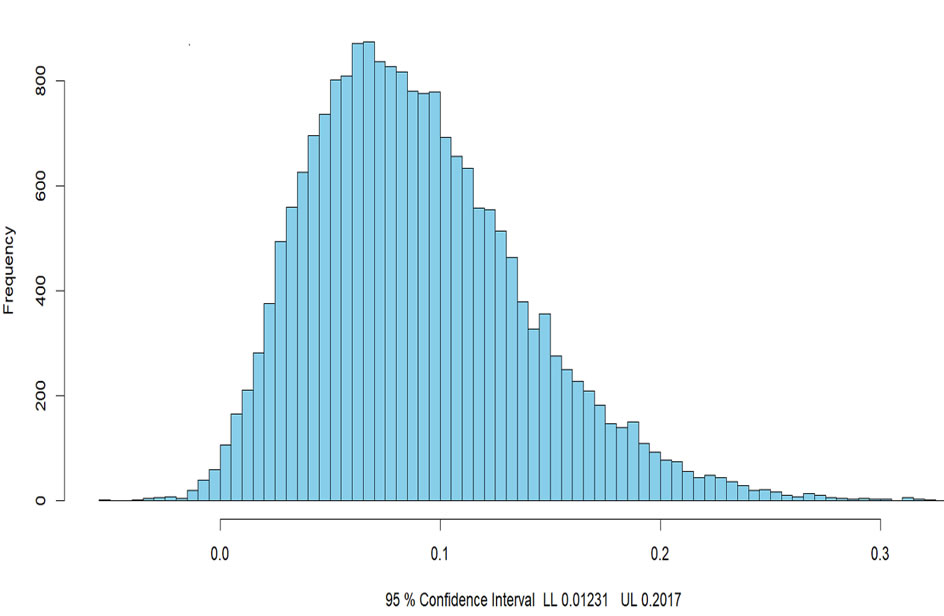
A test, first proposed by Sobel (1982), was initially used to test the indirect effect. Some sources refer to this test as the delta method. The test of the indirect effect is given by dividing ab by the square root of the above variance and treating the ratio as a Z test. This test is very conservative (MacKinnon et al., 1995) because it falsely assumes that the indirect effect has a normal distribution, when in fact it is highly skewed (see figure below). It should no longer be used.
Joint Significance of Paths a and b
If test of a and the test of b are both significant are met, it follows that the indirect effect is nonzero. This simple approach, called the joint significance test, appears to work rather well (Fritz & MacKinnon, 2007), but is rarely used as the definitive test of the indirect effect. (Joint significance presumes that a and b are uncorrelated.) However, Fritz et al. (2012) have strongly urged that researchers use this test in conjunction with other tests. Also, simulation results by Hayes and Scharkow (2013) have shown that this test performs about as well as a bootstrap test. However, Fossum and Montoya (2023) have shown that the test is affected by heteroscedasticity, sometimes being too liberal and other times too conservative. However, the test is not affected by non-normality. Note that the percentile bootstrap test is not affected by non-normality or heteroscedasticity.
This test provides a relatively straightforward way to determine the power of the test of the indirect effect and is used in several programs to compute power. The major drawback with this approach is that it does not provide a confidence interval for the indirect effect.
Bootstrapping
The currently recommended test the indirect effect is bootstrapping (Bollen & Stine, 1990; Shrout & Bolger, 2002). Bootstrapping is a non-parametric method based on resampling with replacement which is done many times, e.g., 5000 times. From each of these samples the indirect effect is computed, and a sampling distribution can be empirically generated. Because the mean of the bootstrapped distribution will not exactly equal the indirect effect a correction for bias can be made. With the distribution, a confidence interval, a p value, or a standard error can be determined. Very typically a confidence interval is computed, and it is checked to determine if zero is in the interval. If zero is not in the interval, then the researcher can be confident that the indirect effect is different from zero. Also, a Z value can be determined by dividing the bootstrapped estimate by its standard error, but bootstrapped standard errors suffer the same problem as the Sobel standard errors and are not recommended. (Bootstrapping does not require the assumption that a and b are uncorrelated.)
Fritz et al. (2012) have raised concerns that bias-corrected bootstrapping test is too liberal with alpha being around .07. Not doing the bias-correction appears to improve the Type I error rate. The current recommendation is to use the percentile bootstrap (bootstrap with no bias correction) and not to use the bias correction (Tibbe & Montoya, 2022).
Several SEM programs (e.g., lavaan, Mplus and Amos) can be used to bootstrap. Also Hayes and Preacher have written SPSS and SAS macros that can be downloaded for tests of indirect effects (click here to download the Hayes and Preacher macro; look for "SPSS and SAS macros to accompany Hayes and Preacher (2010) paper on mediation."). See also the 2022 book by Hayes, which also discusses a bootstrapping macro for the R platform.
Monte Carlo Bootstrap
MacKinnon et al. (2004) and Preacher and Selig (2012) have proposed a computer simulation test of the indirect effect. One starts with the two estimates, a and b, and their standard errors, sa and sb (not the raw data; note sa equals ta divided by a where ta is the t-test for coefficient a). Using this information, random normal variables for a and b are generated to create a distribution of ab values. With these values, confidence intervals and a p value can be created.
Selig and Preacher (2008) have created a helpful program that will perform the necessary calculations using the R package (click here). The test is useful in situations in which there is not easy to bootstrap (e.g., the raw data are unavailable). If estimates of a and b are correlated, then that correlation can be included in the Monte Carlo simulation. Note that distribution above of indirect effects was generated by this app.
Failure to Consider
Causal Assumptions
Statistical mediation analysis is nearly 100 years old. In 1981, Judd and Kenny described the four causal assumptions, mentioned earlier: direction, interaction, reliability, and confounding. The same assumptions were also discussed by James and Brett (1984). In the 1985, Baron and Kenny discussed interaction and reliability, and cited the earlier Judd and Kenny (1981a) paper for more information on the causal assumptions necessary for mediation. So by the mid-1980s the assumptions necessary to draw causal conclusions for mediation were in the literature.
Despite these sources emphasizing the importance of the four causal assumptions, most mediation analysis papers failed to discuss them. Two papers that have carefully examined the extent to which researchers consider those assumptions.
The first is a review by Gelfand et al. (2009) who surveyed mediation studies published in 2002. They took a random sample of 50 of those studies and found the following: Only 1 of the 50 papers mentioned unreliability of M as an issue and only 7 of the 50 mentioned confounding. Most of the papers used cross-sectional data (54%), which likely violated assumptions of causal precedence. The second is a review by Rijnhart et al. (2022) who examined 175 mediation papers published from 2005 to 2009. Only 10% of these papers reported testing for X-M interaction.
Quite clearly most researchers have failed to consider these assumptions. Why is this? I have three ideas why this might be.
The first reason is that for many years psychologists have avoided using causal language and believed that the only way to establish causality was through experimentation. One part of this was reformulating causal modeling of non-experimental data (e.g., Kenny, 1979) and calling it structural equation modeling or SEM (Bentler, 1980). The following quote from Kline (2012) is indicative of this point of view:
Another term that you may have heard is causal modeling, which is a somewhat dated expression first associated with the SEM techniques of path analysis” (p. 8).
But it was not just psychology that moved away from causal terminology. In the early 2000s a biomedical group led by the renowned biostatistician Helena Kramer and funded by the prestigious McArthur Foundation argued that causal terminology not to be used in mediational analyses (Kraemer et al., 2002).
A second reason has to do with the experience of researchers with assumptions in statistical models. Researchers have been taught that multiple regression and analysis of variance were generally robust about assumptions. In particular, violating the normality assumption had little or no effect in the conclusions drawn from those analyses. Researchers did not worry about those assumptions, except when they did not get the results that they wanted. Perhaps this same sort of thinking was mistakenly transferred to the causal assumptions of mediation. The presumption was that mediation analyses were robust over violation of assumptions and could be safely ignored. This is far from the case, as reviewed below.
The third reason is one that has been raised by Causal Inference scholars (e.g., VanderWeele, 2015, p. 26). The most prominent paper discussing the SEM approach to mediation, Baron and Kenny (1986), does not even mention confounding as an assumption. That paper does discuss reliability and interaction and suggests to the reader to consult Judd and Kenny (1981a) for more information about assumptions. The initial submission did discuss confounding, but the editor suggested cutting that section and unfortunately the authors complied. Perhaps, readers of Baron and Kenny (1986) failed to realize the importance of the causal assumptions.
Causal Inference Approach
Click here to see those who helped with this section.
The approach mainly discussed on this page is the SEM approach. A mediation model is proposed involving at least two equations (one for M and another for Y) and the parameters of that model are estimated. An alternative and very different approach has been developed that is usually called the Causal Inference approach. Provided here is a brief and relatively non-technical summary in which attempts to explain the approach to those more familiar with Structural Equation Modeling. Robins and Greenland (1992) conceptualized the approach and more recent papers within this tradition are Pearl (2001; 2011) and Imai et al. (2010). Somewhat more accessible is the paper by Valeri and VanderWeele (2013) and even more accessible is the Book of Why (Pearl & Makenzie, 2018). Valente et al. (2017) have provided a relatively non-technical introduction to this approach. Unfortunately, many who use linear models know relatively little about this approach.
The Causal Inference approach uses the same basic causal structure as the linear approach, albeit usually with different symbols for variables and paths. The two key differences are that the relationships between variables need not be linear, and the variables need not be interval. In fact, typically the variables of X, Y, and M are presumed to be binary, and that X and M are presumed to interact to cause Y. In this literature X is commonly called Exposure and is often symbolized by an A.
The Causal Inference approach is different from SEM in that it focuses on the causal effect of X on Y, and not on the entire model. It does partition that effect into direct and indirect effect. All other effects are of no interest and are included only to improve the estimate of causal effect from X to Y. Alternatively, with SEM the entire model is specified and it must all be true for the model to be valid.
Similar to SEM, the Causal Inference approach attempts to develop a formal basis for causal inference in general and mediation in particular. Typically, counterfactuals or potential outcomes are used. The potential outcome for person i on Y for whom X = 1 would be denoted as Yi(1). The potential outcome of Yi(0) can be defined even though person i did not score 1 on X. Thus, it is a potential outcome or a counterfactual, and not the actual outcome. The averages of these potential outcomes across persons are denoted as E[Y(0)] and E[Y(1)]. To an SEM modeler, potential outcomes can be viewed as predicted values of a structural equation. Consider the structural equation for Y:
Yi= d + cXi + ei
If for individual i for whom Xi equals 1, then Yi(1) = d + c + ei equals his or her score on Y. It can be determined what the score of person i would have been had their score on Xi been equal to 0, i.e., the potential outcome for person i, by taking the structural equation and setting Xi to zero to yield d + ei. Although the term may appear to be new, potential outcomes are not really new to SEM researchers. They simply equal the predicted value for endogenous variable, once the values of its causal variables are fixed.
The Causal Inference approach also employs directed acyclic graphs or DAGs, which are similar though not identical to path diagrams. Moreover, Causal Inference researchers do not use path diagram but DAGs (directed acyclic graphs). They are like path diagrams but usually there are no disturbances or curved lines. A paper by Kunicki et al. (2023) discuss the differences and similarities between DAG and SEM path diagrams.
Assumptions
Earlier, the assumptions necessary for mediation were stated using structural equation modeling terms. Within the Causal Inference approach, the following assumptions about confounding are made:
Condition 1: No unmeasured confounding of the X-Y relationship; that is, any variable that causes both X and Y must be included in the model.
Condition 2: No unmeasured confounding of the M-Y relationship.
Condition 3: No unmeasured confounding of the X-M relationship.
Condition 4: Variable X must not cause any known confounder of the M-Y relationship.
Note that there are ways to avoid Condition 4 that are discussed later on this page. Note also that these assumptions are sufficient but not necessary. That is, if these conditions are met the mediational paths are identified, but there are some special cases where mediational paths are identified even if the assumptions are violated (Pearl, 2014). For instance, consider the case that M ← Z1 ← Z2 → Y but Z1 and not Z2 is measured and included in the model. Note that Z2 is a M-Y confounder and thus violates Condition 2, but it is sufficient to control for only Z1, even though Z1 does not cause Y.
The Causal Inference approach emphasizes sensitivity analysis: These are analyses that ask questions such as, “What would happen to the results if there was a M-Y confounder that had both a moderate effect on M and Y?” As is discussed below, a sensitivity analysis should be an important part of any mediation analysis.
Definitions of the Direct, Indirect, and Total Effects
Because effects involve variables not necessarily at the interval level and because interactions are allowed, the direct, indirect, and total effects need to be redefined. These effects are defined using counterfactuals, not structural equations. Recall from above that for person i, it can be asked: What would person i's score on Y be if person i had scored 0 on X? That value, called the potential outcome, is denoted Yi(0).The population average of these potential outcomes across persons is denoted as E[Y(0)]. The definition of the effect of X on Y or total effect as
E[Y(1)] - E[Y(0)]
This looks strange, but it is useful to remember effects can be viewed as a difference between what the outcome would be when the causal variable differs by one unit. Consider path c in mediation. This difference can be viewed as the difference between what it would be expected that Y would equal when X was 1 and equal to 0, the difference between the two potential outcomes, E[Y(1)] - E[Y(0)].
In the Causal Inference approach, there is the Controlled Direct Effect or CDE for the mediator equal to a particular value, denoted as M (not to be confused with the variable M):
CDE(M) = E[Y(1,M)] - E[Y(0,M)]
where M is a particular value of the mediator. Note that it is E[Y(1,M)] and not E[Y(1|M)], the expected value of Y given that X equals 1 "controlling for M." If X and M interact, the CDE(M) changes for different values of M. To obtain a single measure of the direct effect, several different suggestions have been made. Although the suggestions are different, all of these measures are called "Natural." One idea is to determine the Natural Direct Effect or NDE as follows
NDE = E[Y(1,M0)] - E[Y(0,M0)]
where M0 is the value of M for which X = 0, which is the expected value on the mediator if X were to equal 0 (i.e., the potential outcome of M given X = 0). Thus, within this approach, there needs to be a meaningful "baseline" value for X which becomes its zero value. For instance, if X is the variable experimental group versus control group, then the control group would have a score of 0. However, if X is level of self-esteem, it might be more arbitrary to define the zero value. The parallel Natural Indirect Effect or NIE is defined as
NIE = E[Y(1,M1)] - E[Y(1,M0)]
where M1 is M(1) or the potential outcome for M when X equals 1. The Total Effect becomes the sum of the two:
TE = NIE + NDE = E[Y(1,M1)] - E[Y(1,M0)] = E[Y(1)] - E[Y(0)]
Some readers might benefit from the discussion in Muthén and Asparouhov (2015) on this topic.
Note that both the CDE and the NDE would equal the regression slope or what was earlier called path c' if the model is linear, assumptions are met, and there is no X-M interaction affecting Y, the NIE would equal ab, and the TE would equal ab + c'. In the case in which the specifications made by traditional mediation approach (e.g., linearity, no confounding variables, no X-M interaction), the estimates would be the same.
Given here are the general formulas for the NDE and NIE when X is at the interval level of measurement based on formulas given in Valeri and VanderWeele (2013). If the X-M effect is added to the Y equation, that equation can be stated as
Y = iY + c'X + bM + dXM + EY
and the intercept in the M equation can be denoted as IM. The NDE is
NDE = [c' + d(iM + aX0)](X1 - X0)
and the NIE
NIE = a(b + dX1)(X1 - X0)
where X0 is a theoretical baseline score on X or a "zero" score and X1 is a theoretical "improvement" score on X or "1" score.
When X is a dichotomy, it is obvious what values to use for X0 and X1, the two levels of X. However, when X is measured at the interval level of measurement, there is no consensus as to what to use for the two values. Perhaps, one idea is to use one standard deviation below the mean for X0 and one standard deviation above the mean for X1. Do note that the measure is not in "symmetric" in that if the two are flipped (make X0 be one standard deviation above the mean and X1 be one standard deviation below the mean, the new effects are not the old effects with the opposite sign. Thus, X0 needs to be a "theoretically" low value of X, and in some instances, it might even be the case that X0 is greater than X1.
Meeting the Causal Assumptions of Mediation
Mediation is a hypothesis about a causal network. (See Kraemer et al., 2002) who attempt to define mediation without making causal assumptions.) The conclusions from a mediation analysis are valid only if the causal assumptions are valid (Judd & Kenny, 2010). In this section, the four major assumptions of mediation are discussed. Mediation analysis also makes all the standard assumptions of the general linear model (i.e., linearity, normality, homogeneity of error variance, and independence of errors). It is strongly advised to check these assumptions before conducting a mediational analysis. Clustering effects, which violates the independence assumption are discussed in a later section. What follows are sufficient conditions. That is, if the assumptions are met, the mediational model is identified. However, there are sometimes special cases in which an assumption can be violated, yet the mediation effects are identified (Pearl, 2014).
The focus in these sections is a model in which X is a randomized variable. Thus, the assumption is made that X has no measurement error and there are no confounders of the X-M and X-Y relationship. Should X not be a randomized variable, remedies must be undertaken to remove bias in the effect from X to M and from X to Y.
Direction
To ensure that X is not caused by M or Y, measure X before M and Y. Similarly to make sure that Y does not cause M, measure M before Y). Regarding Y causing M, even if M is measured before Y, it could be that a prior value, one measured before X, which would be a confounding variable.
The mediator may be caused by the outcome variable (Y causing M) , what is commonly called a feedback model. When the causal variable is a manipulated variable, it cannot be caused by either the mediator or the outcome. But because both the mediator and the outcome variables are not manipulated variables, they may cause each other.
If it can be assumed that c' is zero, then a model with reciprocal causal effects can be estimated. That is, if it can be assumed that there is complete mediation (X does not directly cause Y and so c' is zero), the mediator may cause the outcome and the outcome may cause the mediator and the model can be estimated using instrumental variable estimation.
Smith (1982) has developed another method for the estimation of reciprocal causal effects. Both the mediator and the outcome variables are treated as outcome variables, and they each may mediate the effect of the other. To be able to employ the Smith approach, for both the mediator and the outcome, there must be a different variable that is known to cause each of them but not the other. So a variable must be found that is known to cause the mediator but not the outcome and another variable that is known to cause the outcome but not the mediator, an instrumental variable.
I mention here a practice to determine if one has the "correct" causal ordering is to re-estimate the model and switch the variables: Make M the Y variable and Y the M variables. Felix Thoemmes (2015) expains why this strategy of reversing causal arrows is flawed.
Interaction
Judd and Kenny (1981a) and Kraemer et al. (2002) discuss the possibility that M might interact with X to cause Y. Baron and Kenny (1986) refer to this as M being both a mediator and a moderator and Kraemer et al. (2002) as a form of mediation. The X with M interaction should always be estimated and tested and added to the model if present. Judd and Kenny (1981a) discuss how the meaning of path b changes when this interaction is present. Moreover, the Causal Inference approach begins with the assumption that X and M interact and treats the interaction as part of the mediation. In fact, some have argued that the interaction should always be included in the mediation, that is not a position generally taken, nor is it taken here. See VanderWeele (2015, Chapter 9) for a more extended discussion of this issue.
We define the interaction as product of X and M or XM, and denote its effect on Y as d:
M = IM + aX + UM
Y = IY + bM + c'X + dXM + UY
Note that intercepts, IM and IY, are now included in the equations, as well as the interaction or product term, XM. Following, Valeri and VanderWeele (2013) (see also MacKinnon et al., 2020), the Causal Inference definitions of natural indirect effect or the effect of a change in X from X' to X' + 1 on Y due to the effect of X on M with X equal to X' + 1 equals ab + ad(X' + 1); and the natural direct effect or the effect of a change in X from X' to X' + 1 on Y with M equaling IM + aX', equals c' + d(IM + aX'). Note that IM is the intercept from the M equation. Both indirect and direct effects are nonlinear, as X2 becomes a cause of Y.
As an example, consider that the mediation model is M = -1.0 + 0.4X + U Y = 0.0 + 0.3M + 0.12X + 0.12MX + UY
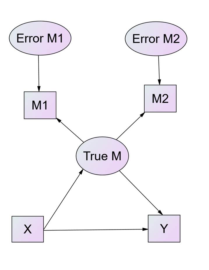
Using the definitions for NIE and NDE, the graph of these effects as function of X is as follows: We first note that both direct and indirect effects increase as X increases, and the rates of increase are the same. Note that when X = 0, there is complete mediation. As X > 0, the is partial mediation. Quite clearly, the presence of interaction in the model greatly complicates the interpretation of direct and indirect effects. Reliability Unreliability is very often present in measurement. Even "hard" measures such as HDL cholesterol are unreliable and a second test a day later is sure to be somewhat different. If the mediator is measured with less than perfect reliability of 1.00, then the effects (b and c') are likely biased. The effect of the mediator on the outcome (path b) is attenuated (i.e., closer to zero than it should be) and the effect of the causal variable on the outcome (path c'') is likely over-estimated if ab is positive and under-estimated when ab is negative. The bias in c' is exacerbated to the extent to which path a is large. If X is measured with less than perfect reliability, then the effects, a and c', are likely biased. The effects of X on M and Y are attenuated, and the effect of the M on Y (path b) is over-estimated if ac’ is positive and underestimated if ac’ is negative. Measurement error in Y does not bias unstandardized estimates, but it does bias standardized estimates, attenuating them. If two or more of the variables have measurement error, the biases are more complicated, as discussed by Cole and Preacher (2014). While not ignored (VanderWeele and Pearl being exceptions) within the Causal Inference approach, biases due to measurement are hardly discussed. When discussed, it is often treated as a form of confounding, where the confounder is true M. Not well-appreciated within the Causal Inference approach is that there are ways of allowing for measurement error in M, something now discussed. If complete mediation can be assumed (a very strong assumption), then instrumental variable estimation can be used. Additionally, the researcher can a priori fix the reliability of M in an SEM analysis (Muthén et al., 2017) or adjust estimates (VanderWeele et al., 2012). Multiple indicators of M within an SEM analysis. Typically, the assumptions made in the measurement model can be tested using an SEM program (e.g., lavaan, Mplus, or Amos). Note the figure below in which there are two indicators of True M (a latent variable), M1and M2. It is assumed that measurement errors are uncorrelated with each other and with true M. The model below can be tested using SEM and has one degree of freedom. Measurement error in Y does not bias the unstandardized estimates of b and c′. It does bias the standardized estimates, an attenuation bias. Treating Y as a latent variable results in a loss of power. Although one obtains less bias by treating the mediator as a latent variable, power can be dramatically reduced. See Hoyle and Kenny (1999) and Ledgerwood and Shrout (2011) for discussions of this issue. To allow for measurement error in M and to allow true M to interact with X, new analytic methods are needed. If X is a dichotomy, then a multiple group SEM can be performed, one model for X= 0 and another for X = 1. If X is continuous, there are methods for latent-variable interactions. See Maslowsky et al. (2015) for a discussion of Klein and Moosbrugger (2000) on how to implement such an analysis. 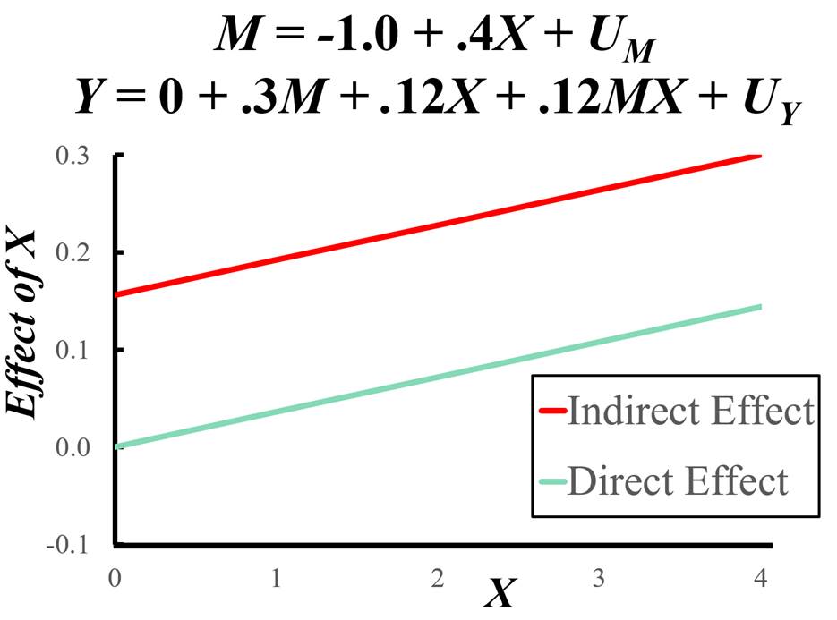
Confounding
Confounding has many different names. Among them are omitted variable, spurious variable, third variable, and selection. In this case, there is a variable that causes both variables in the equation. These variables are called here confounders. For example, a confounder of the M-Y relationship is a variable that causes both the mediator and the outcome. This is the most likely source of specification error and is difficult to find solutions to circumvent it. As noted below, the definition of confounding can be stated more formally and generally.
Discussed in this section are the two different strategies for dealing with confounding: design and analysis. The two design strategies discussed are randomization and holding the confounder constant. Next discussed are statistical strategies and five different strategies are discussed. They are instrumental variable estimation, front-door adjustment, cofounding as the null hypothesis, matching on propensity scores, and inverse propensity weighting. In the next section, it is discussed situations in which a what might be treated as a confounder is not actually a confounder. If the final section, sensitivity analyses are discussed.
Design Strategies
Randomization
One of the best ways to increase the internal validity of mediational analysis is by the design of study, and perhaps the best design feature is the randomizing X (i.e., randomly assigning units to levels of X), By randomizing X, it is known that both M and Y do not cause X. Various researchers (Imai et al., 2013; Spencer et al., 2005) have discussed the randomization of the mediator. Because mediators are often internal variables (e.g., feeling stressed), it can be difficult to find ways to manipulate it.
Hold the Confounder Constant
Often in experimental research, to remove the effects of a confounding variable, the researcher holds a variable constant. If a variable is held constant, it no longer varies and so is no longer a variable and cannot be a confounder. As an example, if a study is planned in an educational setting, a researcher may limit the study to students who are all the same age. In this way, age cannot be a confounding variable. One obvious limitation of such a study is that the results would be limited to that one age. Note that if a variable is held constant, it needs to be potential a confounder and should not be a collider variable or a mediator.
Statistical Strategies
Most often statistical strategies have been used to control for confounding variables. We detail here several such strategies.
Instrumental Variable
An instrumental variable estimation can be used to remove the effects of an unmeasured confounding variable C if one can assume that c' is zero. (See figure below.) In this case, X serves as instrumental variable to estimate the M to Y effect. The instrument must cause M but not Y. Note that M serves as a complete mediator of the X to Y relationship. Instruments must be chosen on the basis of theory not empirical relationships.
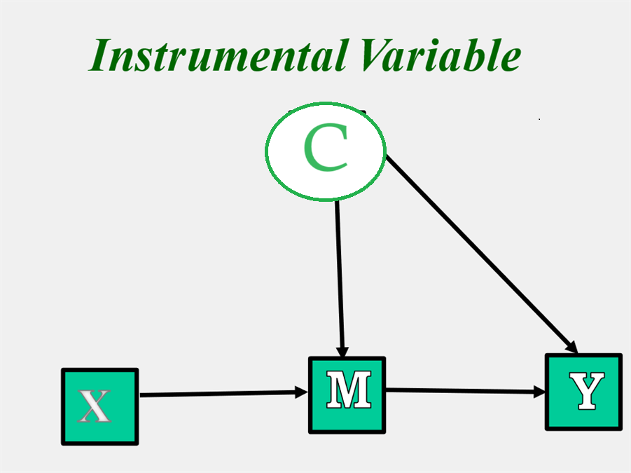
Such a strategy has been suggested, when is M is compliance, a measure of receiving the intervention. Presumably the effect of the intervention is entirely due to the effect of M on Y. In 2021, Joshua Angrist won a Nobel Prize in Economics for applying this strategy.
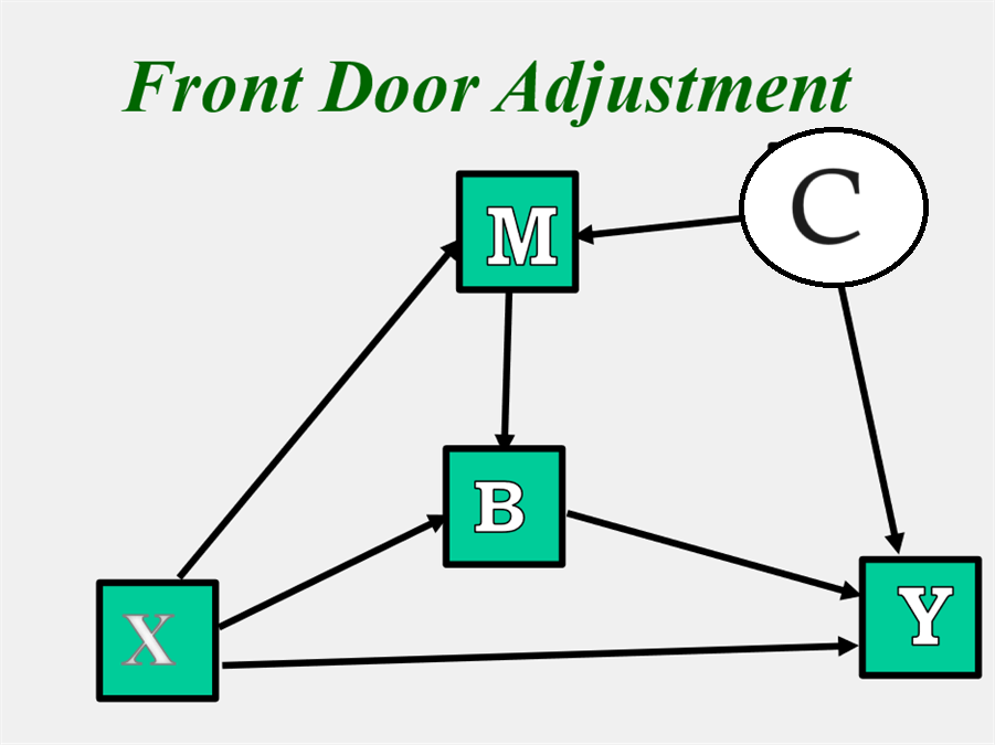
Front-Door Adjustment
Imagine that the same model as above with an instrumental variable, but instead there is a path from X to Y, and thus there is not complete mediation. How could the effect from M to Y be identified? As shown in the figure below, there is a variable B that completely mediates the M to Y relationship but is not affected by C, an unmeasured variable. The indirect effect from M to Y is identified as follows: The path from M to B is identified by regressing B on X and M. The path from B to Y is estimated by regressing Y on X and B. The product of these two paths gives the path from M to Y. The path from X to M is estimated by regressing M on X.
Confounding as the Null Hypothesis
Brewer et al. (1970) argued that in some cases when X is not manipulated, it might be that single unmeasured variable can explain the covariation between all the variables. For mediation, they would be considering the case in which X is a measured, not a randomized variable. For three-variable mediation models, unless there is inconsistent mediation, a single latent variable can always explain the covariation between X, M, and Y (i.e., a solution that converges with no Heywood cases). However, if there are multiple mediators or outcomes, the single-factor model can be ruled out.
This method for ruling out confounding as the source of covariation between variables has to the best of my knowledge has never been used. Nonetheless, I still believe it has potential, which I am currently exploring with my University Connecticut colleague Betsy McCoach.
Multiple Regression or Analysis of Covariance Adjustment
The most often used strategy to remove the effects of confounding variables is to include those variables in the analysis as covariates, what Pearl and Mackenzie (2018, pp. 158-159) call backdoor path. There are two potential difficulties with this strategy: p hacking and low power.
The p hacking problem is the practice of a researcher either consciously or unconsciously selecting a particular combination of covariates to show a desired result. To guard against such a practice, the researcher should preregister the strategy for the inclusion and exclusion of covariates in the model.
Low power is also a consideration. Often studies have a large number of potential covariates and when one allows for nonlinear effect and covariate interactions with each other, there can be a dramatic loss in power if all such variables are included in the analysis.
Inverse Propensity Weighting
This method, also called inverse probability weighting or marginal structural models, was initially proposed by Robins and colleagues (Robins et al., 2000). The basic idea, as the name suggests, is that by re-weighting the analysis using propensity scores, the effects of confounding can be removed.
Propensity scores were originally proposed by Rosenbaum and Rubin (1983) and can be viewed as a way of creating a multivariate match in observational studies. Assuming that X is a 0-1 dichotomy (0 = control, 1 = treated) and not randomized. A logistic regression on X using the set of covariates as predictors is run. From that logistic regression, the predicted X values are obtained, and are called propensity scores, which can be viewed as the probability that the person is in the treated group (i.e., X = 1) given the set of potential confounders, i.e., covariates. Inverse propensity weighting is the idea using propensity scores to re-weight the analysis to reduce the effect of confounding.
To illustrate the method, consider the effect of M, a dichotomy, on Y, ignoring X. The propensity score for person i using logistic regression with the set of covariates to predict M is denoted as Pi. Using propensity scores, weights for the analysis are computed as follows: For M = 1, compute the weight as P(M = 1)/Pi, and for M = 0, compute the weight as P(M = 0)/(1 - Pi). By weighting in this way, the confounding effects of the covariates can be removed.
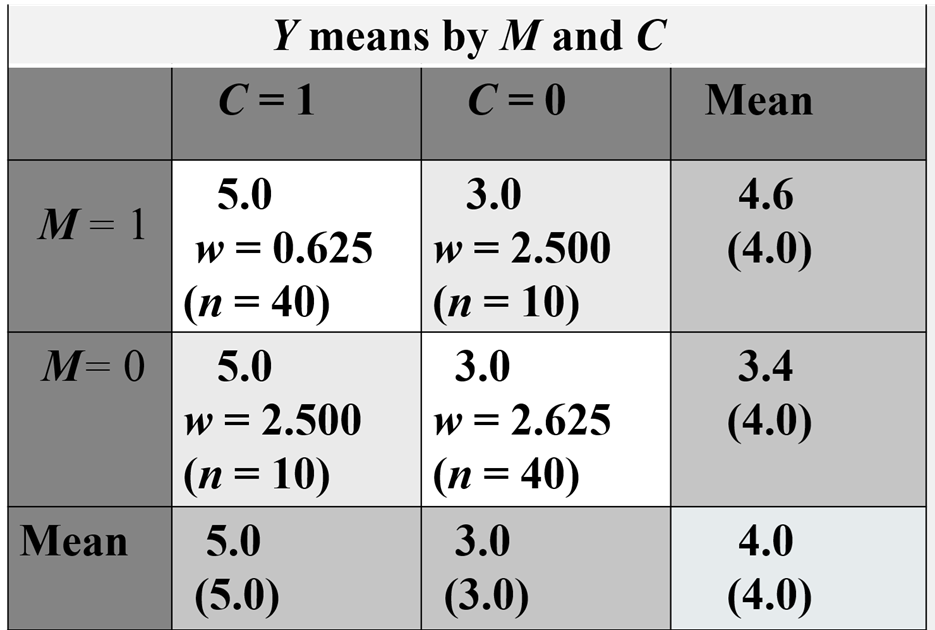
To help in understanding how weighting can remove bias due to confounding, consider an example of M’s effect of Y, where M is a dichotomy {0,1}. The variable M has no effect on Y once a dichotomous confounder, C, is controlled. As seen in the table below, if C is ignored, the mean of Y when M = 1 is 4.6, and the mean of Y when M = 0 is 3.4, a difference of 1.2 units. However, looking within levels of C, there is no difference in means between M1, and M0; when C = 1, the M1, and M0 means are both 5.0, and when C = 0, both means equal 3.0. If inverse propensity weights are computed, the weights in the two diagonal cells are 0.625 (.5/.8) and in the two off-diagonal cells are 2.500 (.5/.2). What these weights do is effectively weight all four cells equally giving them an N of 25 and unconfounds M and C. Using these weights in a weighted regression analysis results in an estimate of the effect of M on Y of 0.00, the proper value. Note before reweighting, the correlation between M and C was .8. But by reweighting, that correlation becomes zero.
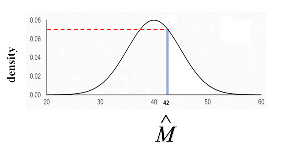
Very often the variable M is not be a dichotomy and also M may be caused by X. To compute the propensity score, it is typically assumed that M has a normal distribution. First computed is predicted value M (M-hat) given a set of predictors. The propensity score is defined as the density M given the set of covariates and X. To help understand what the density is, consider the figure below. It contains a probability function for a normally distributed variable with a mean of 40 and a standard deviation of 5. For a given M-hat, or predicted Y, 42 in the figure, the point where it intersects the normal curve (the blue line) is determined and a horizontal line (dashed red line) is drawn to determine its density. Density is the analog to probability for continuous distributions like the normal.
For mediation analysis in which the concern is M-Y confounders and M is continuous, the weights are computed as follows. The numerator is the density of M, assuming a normal distribution, given M. The denominator is density of M and the set of confounders. The R code for computing these weights is given in Heiss (2020).
It is also advisable to combine inverse propensity weighting with including as covariates strong predictors of Y. Such a procedure is said to be doubly robust. For an illustration of inverse propensity weighting, see Valente et al. (2017).
A major difficulty with inverse propensity weighting, especially with a continuous mediator, is that often the weights are very extreme creating problems in the estimation (Li & Li., 2019).
Strong Assumptions
Two different strategies had been outlined for the removal of the effects of confounding: multiple regression (sometimes called analysis of covariance) and inverse propensity weighting. It is important to realize that these strategies assume that ALL the confounding variables are assumed to be included in the set of covariates. It is called strong ignorability by Rubin and exchangeability by Robins. These methods also assume that all the covariates are measured without error (Steiner et al., 2011; Westfall & Yakoni, 2016). Moreover, these methods do not take care of unreliability in the mediator. A reasonable expectation is that they these methods would typically remove only some but not all of the effects of confounding. That is why sensitivity analyses are strongly recommended, which are discussed below.
Some Confounders May Not Be Confounders
Researchers need to be careful about what variables are treated as confounders. As is discussed in the following sections, problems can arise if the wrong variables are treated as confounders. Discussion focuses on M-Y confounders.
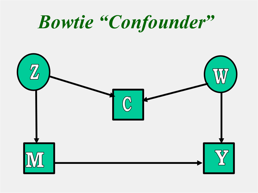
Bowtie Confounders
Note the definition of a confounder is a variable that causes both M and Y but not just correlated. Note in the figure below, C is correlated with M and Y but does not cause either and so would not be treated as confounder. The example is taken from Pearl (2000, p. 186) and is called "bowtie" because the picture looks like a bowtie.
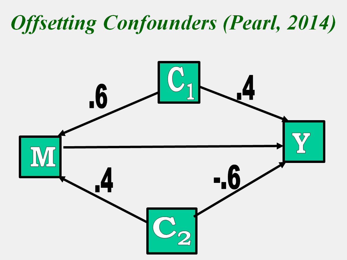
Offsetting Confounders
In the case below, there are two confounders, C1 and C2. But note that is this case, there two effects offset each other, one with a standardized effect of .24 and with -.24. Note that if C1 was "controlled," the M to Y effect would be negatively biased, and if C2 was controlled, it would be positively biased. In this case, controlling for a confounder, biases the estimate. For this and other reasons, it is not necessary to control for all confounders. What the figure illustrates is that although C1 and C2 are confounders, there is no need to control for them in this case. For a detailed explanation of the rules for controlling for confounders, consult Pearl (2014).
Collider and Mediating Variables
A collider variable is a variable that is caused by M and Y and so their two paths “collide” in causing Y. See Rohrer (2018) for a discussion of collider variables. Note if the researcher holds a collider constant that too leads to problems. For instance, if there was a study that examined the effects of surgery on a patient’s outcome (e.g., heart function), but the study only examined patients who survived, survival would be a collider variable.
A mediator too should not be treated as a confounder. However, sometimes, as discussed in the next section, a post-treatment confounder can be treated as mediator.
Post-treatment Confounders: G Estimation
As was discussed in the Causal Inference section, one assumption is that there does not exist a post-treatment confounder C of the M-Y relationship that is caused by X (Condition 4). Note below that C is caused by X, and causes M and Y. Such a variable has been called a post-treatment or intermediate confounder. The red path indicates a path from X to the confounder.
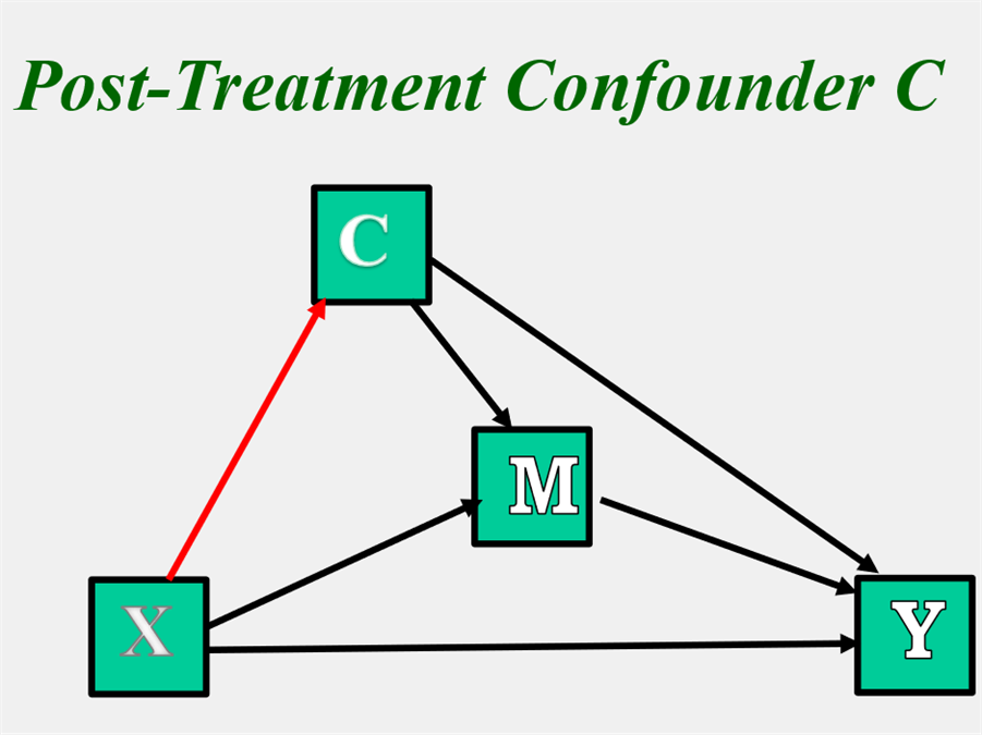
Note that the "confounder" C could alternatively be interpreted as a second mediator. If it was treated as such, there would be three indirect effects: one through C (X → C → Y), one through M (X → M → Y), and one through C and M (X → C → M → Y). The model is identified. However, if for some reason, researchers may not want to treat C as a mediator, but as a confounder. If so, the indirect effect of X on Y via C (X → C → Y) would be treated as part of the direct effect of X on Y and the indirect effect of X on Y via C and M (X → C → M → Y) would be treated as part of the indirect effect of M. The model is still identified, but It is my understanding that this formulation makes it impossible to define the natural indirect effect of X on Y via only M using potential outcomes (see VanderWeele, 2015), which is why the Condition IV is needed. If instead, C is treated as a second mediator, there is no problem.
We can add an additional complication to the above model, by adding an unmeasured confounder that causes X, C, and Y, but not M. Thus, C is assumed to mediate the effect of the unmeasured confounder on M. This new model is under-identified. However, there is a way to estimate the indirect and direct effects of X on Y via M and treating C as a confounder using G estimation, described in several papers by Vansteelandt (e.g., Moerkerke et al., 2015) and involves three steps:
1. Estimate the total effect or c, by regressing Y on X.
2. Treat Y as the outcome with X, M, and C as predictors. The coefficient for M is denoted as b0. Compute Y - b0 and call it Y'.
3. Treat Y' as the outcome with X as the only predictor. This last step gives c'. Estimate ab from c - c'.
Note that G estimation estimate of the direct effect includes the C indirect effect (X → C → Y), and the estimate of the indirect effect includes the C to D indirect effect (X → C → D → Y). Illustrations of G estimation include Moerkerke et al. (2015), Loeys et al. (2014), Valente et al. (2017), and Kisbu-Sakarya et al. (2020).
Sensitivity Analyses
As discussed above, it is often assumed for mediation that there is perfect reliability for X and M, no omitted variables for the X to M, X to Y, and M to Y relationships, and no causal effects from Y to X and M and from M to X. It is possible to determine what would happen to the mediational paths if one or more of these assumptions is violated by conducting sensitivity analyses. For instance, one might find that allowing for measurement error in M (reliability of .8) that path b would be larger by 0.15 and that c' would be less by 0.10. Alternatively, one might determine what was the value of reliability that would make c' equal zero. A thorough mediation analysis should be accompanied by a sensitivity analysis.
One way to conduct a sensitivity analysis is to estimate the mediational model using SEM (Harring et al., 2017). Consider a sensitivity analysis allowing for a possible unmeasured confounder of the M to Y relationship. One can either create a phantom variable C, with a fixed variance (usually one) and fixed paths to M and Y (Mauro, 1990). Imai, Keele, and Yamamoto (2010) have suggested a different but equivalent strategy of just allowing for a correlation in the disturbances of M and Y.
One fixes the additional parameter to the value of interest. For example, an omitted variable is added that has a moderate effect on M and Y. One can then use the estimates from this analysis in the sensitivity analysis.
Note that if the causal variable, X, is randomized, then omitted variables do not bias the estimates of a and c. However, in this case, paths b and c' might be biased if there is an omitted variable that causes both M and Y. Assuming that this omitted variable has paths in the same direction on M and Y and that ab is positive, then path b is over-estimated and path c' is underestimated. In this case, if the true c' were zero, then it would appear that there was inconsistent mediation when in fact there is complete mediation.
Fritz et al. (2017) point out that in the case in which X is manipulated and M has measurement error and there is a confounder for M and Y, it can happen that the two biases can to some degree offset each other. That is, assuming a and b being positive, measurement error in M in this case leads to under-estimation of b and over-estimation of c' whereas typically (but not always) a M-Y confounder leads to over-estimation of b and under-estimation of c'. See the paper for details and an example.
Current State of Mediational Analysis
Data Analysis
Multiple Regression
Traditionally, the linear mediation model is estimated by estimating a series of multiple regression equations. Minimally two equations, one for M and one for Y, need to be estimated.
The major difficulty is in the testing of the indirect effect for statistical significance. Several possibilities are available. Discussed earlier are Monte Carlo bootstrap and the joint significance test. Another alternative is to use PROCESS, which has macros (add-ons) for SPSS, SAS, and R that perform bootstrap analyses. For more details on PROCESS consult Hayes (2022).
Structural Equation Modeling
There are considerable advantages to estimate the program using a Structural Equation Modeling (SEM) program, such as Amos, Mplus, or lavaan (Iacobucci et al., 2007). First, all the coefficients are estimated in a single run. Second, most SEM programs provide estimates of indirect effects and bootstrapping. Third, SEM with FIML estimation can allow for a more complex model of missing data. Fourth, it is relatively easy to conduct sensitivity analyses with a SEM program. Fifth, one can include latent variable and reciprocal causation with an SEM program.
Normally with SEM, one computes a measure of fit. However, the basic mediational model with no latent variables is saturated and the usual measure of fit (e.g., RMSEA and CFI) cannot be computed (i.e., the degrees of freedom of the model are zero). However, one can adopt the following strategy. Use a fit statistic an "Information" measure like the AIC or BIC. I prefer the SABIC which, at least in my experience, performs better than the other two. With these information measures, a fit value can be obtained for a saturated model. Then one can compute the measure for each of the following models: no direct effect, no effect from causal variable to the mediator, and no effect from the mediator to outcome. The best fitting model is the one with lowest value.
Causal Inference Software
As reviewed by Valente et al. (2020), there are several programs that provide estimates of effects using the Causal Inference approach. That review highly recommends Mplus and the CAUSALMED procedure within SAS (click here). Since the publication of review, Stata 18 has added a causal mediation analysis (click here).
Valente et al. (2020) recommend two R packages for mediation. One, called mediation (Tingley et al., 2014) is authored by the Imai group and allows for sensitivity analyses. To read an extended illustration of this package see the Chi et al. (2022) paper. The second recommended R package is the Ghent group's medflex (Steen et al., 2017).
The R platform has numerous other packages to assist in mediation analysis. Two notable ones are ipw (van der Wal & Geskus (2011), which does inverse proportional weighting and MBES, written by Ken Kelley (effect sizes for mediation; Preacher & Kelley, 2011).
Reporting Results
Mediation papers need to report the indirect effect and its confidence interval. Additionally, the paths a, b, c, and c', as well their statistical significance (or confidence interval) are reported. Although some have suggested not drawing conclusions about complete versus partial mediation, it seems something that is reasonable, although one must be careful about the relatively low power of tests the total and direct effects.
It is essential that one discuss the likelihood of meeting the assumptions of mediational analysis and ideally reporting on the results of sensitivity analyses. (See discussion below.) See the paper by Yzerbyt et al. (2018) on reporting results of mediational analyses.
Power
The indirect effect is the product of two effects. One simple way, but not the only way, to determine the effect size is to measure the product of the two effects, each turned into an effect size. The standard effect size for paths a and b is a partial correlation; that is, for path a, it is the correlation between X and M, controlling for the covariates and any other Xs and for path b, it is the correlation between M and Y, controlling for covariates and other Ms and Xs. One possible effect size for the indirect effect would be the product of the two partial correlations. (Preacher and Kelley (2011) discuss a similar measure of effect size which they refer to as the completely standardized indirect effect, which uses betas, not partial correlations.)
There are two different strategies for determining small, medium, and large effect sizes. (Any designation of small, medium, or larger is fundamentally arbitrary and depends on the particular application.) First, following Shrout and Bolger (2002), the usual Cohen (1988) standards of .1 for small, .3 for medium, and .5 for large could be used. Alternatively, and I think more appropriately because an indirect effect is a product of two effects, these values should be squared. Thus, a small effect size would be .01, medium would be .09, and large would be .25. Note that if X is a dichotomy, it makes sense to replace the correlation for path a with Cohen’s d. In this case the effect size would be a d times an r and a small effect size would be .02, medium would .15, and large would be .40.
Distal and Proximal Mediators
In this section, it is presumed that paths a and b are positive, something that can always be accomplished by reversing X or M or both. To demonstrate mediation both paths a and b need to be present. Generally, the maximum size of the product ab equals a value near c, and so as path a increases, path b must decrease and vice versa. Hoyle and Kenny (1999) define a proximal mediator as path a being greater than path b (all variables standardized) and a distal mediator as b being greater than a.
A mediator can be too close in time or in the process to the causal variable and so path a would be relatively large and path b relatively small. An example of a proximal mediator is a manipulation check. The use of a very proximal mediator creates strong multicollinearity which lowers power as is discussed in the next section.
Alternatively, the mediator can be chosen too close to the outcome and with a distal mediator path b is large and path a is small. Ideally in terms of power, standardized a and b should be comparable in size. However, work by Hoyle and Kenny (1999) shows that the power of the test of ab is maximal when b is somewhat larger than a in absolute value. So slightly distal mediators result in somewhat greater power than proximal mediators. Note that if there is proximal mediation (a > b), sometimes power actually declines as a (and so ab) increases.
Multicollinearity
If M is a successful mediator, it is necessarily correlated with X due to path a. This correlation, called collinearity, affects the precision of the estimates of the last regression equation. If X were to explain all of the variance in M, then there would be no unique variance in M to explain Y. Given that path a is nonzero, the power of the tests of the coefficients b and c’ is lowered. The effective sample size for the tests of coefficients b and c’s approximately N(1 - r2) where N is the total sample size and r is the correlation between the causal variable and the mediator, which is equal to standardized a. So, if M is a strong mediator path a is large), to achieve equivalent power, the sample size to test coefficients b and c' would have to be larger than what it would be if M were a weak mediator. Multicollinearity is to be expected in a mediational analysis and it cannot be avoided.
Low Power for Tests of c and c'
As described by Kenny and Judd (2014), as well as others, the tests of c and c’ have relatively low power, especially in comparison to the indirect effect. It can easily happen, that ab can be statistically significant but c is not. For instance, if a = b = .4 and c' = 0, making c = .16, and N = 100, the power of the test of path a is .99, the power of the test of path b is .97 which makes the power of ab equal to about .96, but the power of the test that c is only .36. Surprisingly, it is very easy to have complete mediation, a statistically significant indirect effect, but no statistical evidence that X causes Y ignoring M.
One way of understanding this power advantage in testing ab over c' is that the test ab is essence the combination of two tests. Testing c' is like being to kick a football 100 meters, whereas the test of ab is like kicking it 50 meters. Because the two effects multiple, it more like being about to kick it 16 meters.
Because of the low power in the test of c’, one needs to be very careful about any claim of complete mediation based on the non-significance of c’. In fact, several sources (e.g., Hayes & Scharkow, 2013) have argued that one should never make any claim of complete or partial mediation. Alternatively, such claims can be made, but caution is in order. Minimally, there should be sufficient power to test for partial mediation, i.e., have enough power of the test of c' . However, if the sample size is very large, then finding a significant value for c' is not very informative. More informative, in the case of large N studies, is knowing the proportion of the total effect that is mediated or ab/c. Note also, that finding that c' equals zero does not prove complete mediation. There may well be an additional unmeasured mediator, making what was complete mediation partial mediation.
Power Program and Apps
Discussed here are two apps and one power program that can be used to forecast the power of the test that the indirect effect is zero. The programs can also be used to forecast the minimum sample size needed to achieve a desired level of power or the sample size needed to achieve the desired level of power. Alternatively, and more generally, one could use a structural equation modeling to run a simulation to conduct a power analysis.
MedPower. One strategy to compute the power of the test of the indirect effect is to use the joint test of significance. Thus, one computes the power of test of paths a and b and then multiplies their power to obtain the power of the test of the indirect effect. One can use the app called MedPower (Kenny, 2017) to conduct a power analysis. The opening screen of the app is:
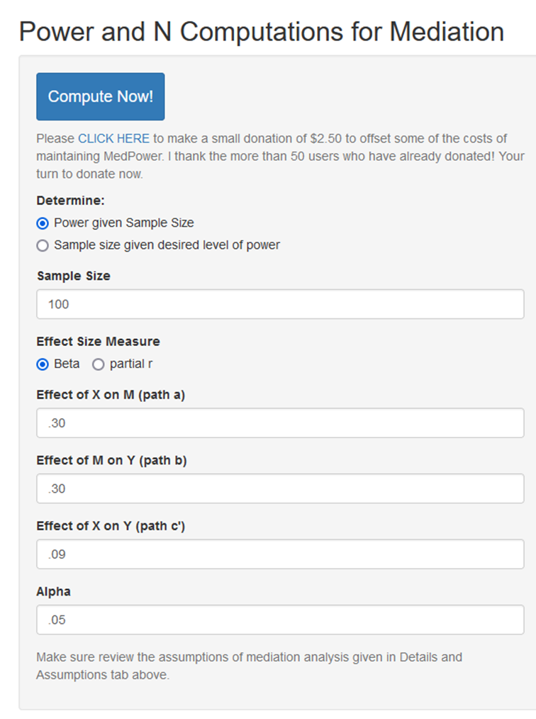
The user can either find the power given the sample size, or the sample size needed given the effect sizes. In the above example, effect sizes are standardized values, beta coefficients. The output from these choices are as follows:
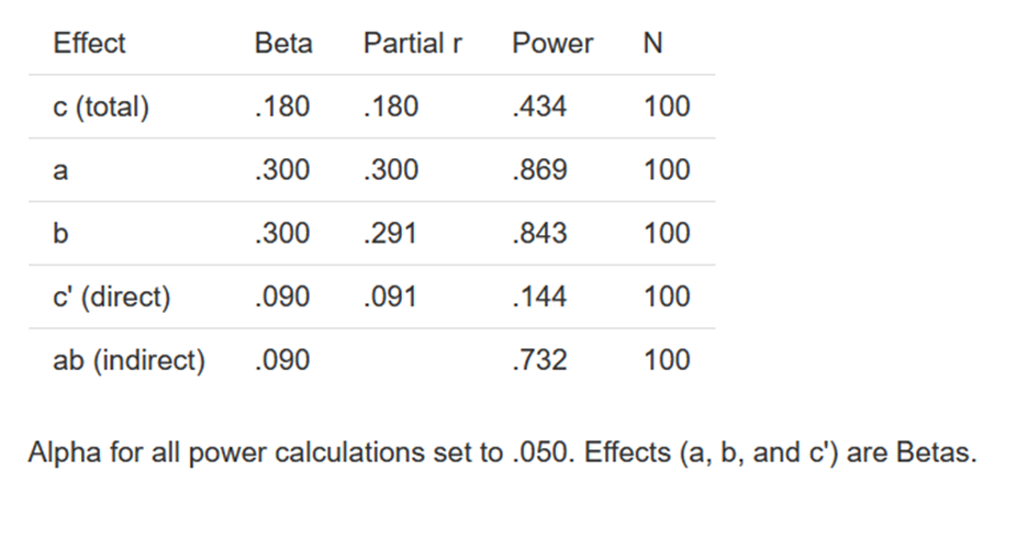
Note that the estimate of the power for the indirect effect is .732, which is much larger than the power of the direct effect, which is the same value, .090, as the indirect effect.
mc_power_med. The program Monte Carlo Power Analysis for Indirect Effects (Schoemann et al., 2017) is also a shiny program. Unlike MedPower, this program uses a Monte Carlo bootstrap. Moreover, while MedPower is limited to a single X and M, this program is more flexible and there can be multiple M variables.
The website to access the program is schoemanna.shinyapps.io/mc_power_med/. The same values for a, b, c' and N as were inputted as were for MedPower and the following result was obtained:
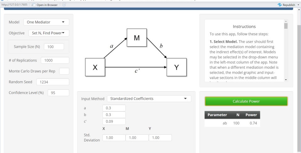
Only the power for the test of indirect effect is given and it equals .74, not all that different from the MedPower value of .732. Consistent with prior reseach, bootstraping and joint significance yield similar results.
pwr2ppl. This is an general R package to compute power (Aberson, 2019) and has the catchy name of pwr2ppl, echoing the 1971 John Lennon song of "Power to the People." To install the package in R one needs to enter:
install.packages("pwr2ppl”)
The program allows for up to four X variables and four mediators. It inputs correlations, and not betas. Power is computed for only the indirect effect. Like MedPower it uses a joint significance test, but it runs a simulation. The program does allow for multiple X, M, and Y variables. Here is what is obtained for running example:
pwr2ppl::medjs(rx1m1= .30,rx1y = .18,
rym1 = .3 + .3*.09,n = 100,
alpha = 0.05, mvars=1,
rep = 10000)
power = .7297
Note all three methods of estimating power yield essentially the same result.
Criticism of Mediation Analyses and the Response
Not surprisingly, given the low rate that mediation researchers consider causal assumptions (see above) and given the increasing awareness of the importance of causal assumptions due to the emergence of Causal Inference approach, it is hardly surprising that some are highly critical of mediation analyses that fail to discuss and try to satisfy the causal assumptions. Here, those criticisms are reviewed and how they might be handled.
One concern raised by Cole and Maxwell (2007) and Cole et al. (2012) is that mediational analyses of cross-sectional studies very often yields invalid estimates of mediational effects. Very rarely cross-sectional mediation analyses are informative; possible only with strong assumptions about X and M being retrospective or stable measures Take note of the point made by Kenny (2019):
Certainly, an uncritical use of a cross-sectional design is problematic, but not always fatal, a point
alluded to by Maxwell and Cole (see p. 40). Consider the study by Riggs et al. (2011). They were interested in the mediating effect of attachment styles of
both oneself and one’s relationship partner, which mediated the causal effect of childhood abuse on relationship satisfaction. They measured all of these variables from 155 heterosexual couples at one time. The authors presented evidence of the validity of retrospective measures of childhood
abuse (see pp. 134–135). There is the worry that relationship satisfaction might affect attachment style, but
likely, the preponderance of the causation goes from attachment to satisfaction. Thus, in this case, a cross-sectional mediation analysis is not as problematic as it might seem (p. 1022).
Smith (2012) in his editorial in the Journal of Personality and Social Psychology argued that mediational analyses made strong assumptions that were rarely fully met and so conclusions from mediational analyses should be very cautious. Also notable, Rex Kline in 2015 noted what he called three myths or bad practices in mediational analyses. Finally, a recent paper by Rohrer et al. (2022) noted that many of the papers that used by PROCESS (Hayes (2022) failed to explicitly discuss the underlying causal assumptions. Note that although all of the above sources are highly critical of the current practice of mediational analysis, none of those sources do not advocate never conducting mediational analysis. They do not argue that mediational analyses should never be done, but rather if they are done, they need to be done well. Moreover, despite these criticisms, mediation analyses are still extremely popular. In fact, by one measure (citations of Baron & Kenny, 1986), the number of published mediators papers increased by 16% from 2012 to 2021 over the prior 10 years.
Rohrer et al. (2022) has an excellent discussion of what is needed in mediational analyses:
(A)uthors should list the actual specific assumptions under which their central estimate of the causal effects can be interpreted: This estimate corresponds to the causal effect of X and Y under the assumption that … there are no common causes between the two of them …. Such assumptions may often appear unrealistic, but they can be supplemented with statements about the degree to which conclusions are sensitive to violations of these assumptions (p. 17).
It should also be noted besides confounding, researchers need to pay attention to other assumptions of causal mediation analysis, most notably unreliability of the causal variables.
One way to increase awareness of the causal assumptions of mediation analyses for authors, reviewers, editors, and consumers is to have a checklist of relevant issues. Along these lines, Lee et al. (2021) in the Journal of the American Medical Association provide a checklist of things to do. Among them are the following:
Specify assumptions about the causal model.
Specify analytic strategies used to reduce confounding.
Interpret the estimated effects considering the study’s magnitude and uncertainty, plausibility of the causal assumptions, limitations, generalizability of the findings.
Like other sources, Lee et al. emphasize confounding, but they fail to discuss in much detail the importance of assumption of no measurement error in causal variables.
Mediation analyses remain popular, even though they are difficult to do. If we are to have a science examining the causal effects of variable that cannot or should not be manipulated, we need to develop such methods (Grosz et, al., 2020; Rohrer, 2018).
Briefly Discussed Topics
Several topics have not been discussed. A brief discussion of several of them is provided with relevant references.
X Within-Participants
In these studies each participant is in the experimental and control group and M and Y are measured for both conditions. Judd et al. (2001) discuss a generalization of repeated measures analysis of variance test of mediation. Work by Montoya and Hayes (2017) has extended that analysis to include the measurement of the indirect effect.
Multiple Causal or X Variables
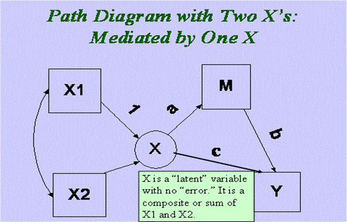
In this case there are multiple X variables and each has an indirect effect on Y. An SEM program can be used to test hypotheses about the linear combinations of indirect effects: For example, are they equal? Do they sum to zero?
One can alternatively treat the multiple X variables as a formative variable and so if a single “super variable” can be used to summarize the indirect effect. As seen below, the formative variable X “mediates” the effect of X on M and Y. The model can be tested and it has k - 1 degrees of freedom where k is the number of X variables. Thus, the degrees of freedom for the example would be 1.
Multiple Mediators
If there are multiple mediators, they can be tested simultaneously or separately. The advantage of doing them simultaneously is that one learns if the mediation is independent of the effect of the other mediators. One should make sure that the different mediators are conceptually distinct and not too highly correlated. [Kenny et al. (1998) considered an example with two mediators.]
Sometimes the mediators are causally ordered and are said to form a mediational chain. See Taylor et al. (2008) for a discussion of the estimation of this type of model.
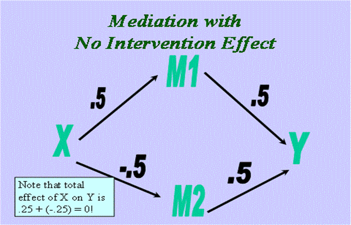
There is an interesting case of two mediators (see below) in which the indirect effects are opposite in sign. The sum of indirect effects for M1 and M2 would be zero. It might then be possible that the total effect or c is near zero, because there are two indirect effects that work in the opposite direction. In this case "no effect" would be mediated. The case in which there are two indirect effects of the same effect that are approximately equal in size but opposite in sign might be called offsetting mediators. Examples of opposing mediators in the literature of offsetting mediators are in Salthouse (1984) and Richards and Banas (2018). It is also possible to find offsetting mediators in program evaluation. There might be two different interventions, A and B, that work though two different mechanisms, M1 and M2. If X is a dummy variable that compares the two different interventions and both interventions are mediated by their proposed mechanism, the pattern would be offsetting mediators.
One can test hypotheses about the linear combinations of indirect effects: For example, it can be if they are equal or if they sum to zero. Ledermann et al. (2011) consider various contrasts of indirect effects in studies of dyadic mediation.
Multiple Outcomes
If there are multiple outcomes, they can be tested simultaneously or separately. If tested simultaneously, the entire model can be estimated by structural equation modeling. One might want to consider combining the multiple outcomes into one or more latent variables. Alternatively, the outcomes have their own causal structure, the model should be considered as a mediational chain.
Covariates
There are often variables that do not change that can cause or be correlated with the causal variable, mediator, and outcome (e.g., age, gender, and ethnicity); these variables are commonly called covariates. They take on a dual role in mediation analyses. They might be potential confounds, as was discussed above. Alternatively, they may explain variation in the outcome and increase the power in the analysis. They would generally be included in the M and Y equations. When conducting multiple regression analyses, a covariate would not be trimmed from an equation unless it is dropped from all of the other equations. If a covariate interacts with X or M, it would be treated as a moderator variable.
Mediated Moderation and Moderated Mediation
Moderation means that the effect of a variable on an outcome is altered (i.e., moderated) by a covariate. (To read about moderation click here.) Moderation is usually captured by an interaction between the causal variable and the covariate. If this moderation is mediated, then there is the usual pattern of mediation but the X variable is an interaction and the pattern would be referred to as mediated moderation. The total effect or the original moderation effect could be computed, as well as the direct effect or how much moderation exists after introducing the moderator, and the indirect effect or how much of the total effect of the moderator is due to the mediator.
Sometimes, mediation can be stronger for one group (e.g., males) than for another (e.g., females), something called moderated mediation. There are two major different forms of moderated mediation. The effect of the causal variable on the mediator may differ as a function of the moderator (i.e., path a varies) or the mediator may interact with the moderator to cause the outcome (i.e., path b varies). It is also possible that the direct effect or c’ might change as a function of the moderator.
Papers by Muller et al. (2005) and Edwards and Lambert (2007) discuss mediated moderation and moderated mediation and examples of each. Muller et al. (2005) explains the difference between moderated mediation and mediated moderation. Also Preacher et al. (2007) have developed a macro for estimating moderated mediation. Finally, the Schoemann et al. (2017) app can be used to conduct power analyses for moderated mediation.
Clustered Data
Traditional mediation analyses presume that the data are at just one level. However, sometimes the data are clustered in that persons are in classrooms or groups. With clustered data, multilevel modeling is often recommended. Estimation of mediation within multilevel models can be very complicated, especially when the mediation occurs at level one and when that mediation is allowed to be random, i.e., vary across level two units. The reader is referred to Krull and MacKinnon (1999), Kenny et al. (2003), and Bauer et al. (2006) for a discussion of this topic. Preacher et al. (2010) have proposed that multilevel structural equation methods or MSEM can be used to estimate these models. Ledermann et al. (2011) discuss mediational models for dyadic data, which may have as many as eight indirect effects.
Longitudinal Data
Sometimes there are studies in which participants are measured a few times, perhaps as few as twice. An introduction to this topic is in Roth and MacKinnon (2012). See also Chapter 6 in VanderWeele (2015).
In principle, having a baseline measure of M and Y might be a way of control for confounders. Consider the case of estimating the effect from X to M, where X is not a randomized variable, and there is a baseline measure of M, denoted as M0. Following Judd and Kenny (1981b, Chapter 5), the key issue is what is assumed about the relationship between M0 and S, where S is the variable that determines the non-random assignment to levels of X.
First, one could treat M0 as a complete mediator of S-M relationship: X ←S → M0 → M. [This is a case where the confounder S is unobserved, but it causes M0 and M0 can serve as a proxy for S (Pearl, 2012)]. If this assumption is true one could either control for M0 or treat it as a confounder using inverse propensity weighting. Likely too, one would also need to make adjustments for measurement error M0.
Second, one could assume that S does not change during the study and that its effect on M and M0 is stationary. If so, then using a simple difference score would remove the confounding effect of S. Such an analysis has been called a difference of differences in economics. See also the paper by Kim and Steiner (2021) that presents DAG representation of this approach.
The fact that these two different strategies yield difference answers is often referred to as Lord's paradox (Lord, 1967). It illustrates that having baseline measures does not solve the confounding problem. Further documentation of the difficulties of drawing causal inference from longitudinal data can be seen in the analysis of Usami et al. (2019), seven very different approaches to the estimation of causal effects from multiwave studies are presented.
Intensive Longitudinal Data
In this form of analysis there are many time points, as in the case of diary studies. These studies can be treated as clustered data, but there are further complications due to temporal nature of the data. Among such complications are correlated errors, lagged effects, and the outcome causing the mediator. One possibility for analysis is DSEM (McNeish & MacKinnon, 2022), which is an option in Mplus that uses Bayesian analysis.
Conclusion
Mediation analyses continue to be a topic of intense interest because they provide answers to important research questions. This page has focused on the difficulties in mediation analyses, but it is important to not lose sight that mediation analyses have provided important information about causal processes. Mediational analyses have advanced our understanding in many areas, e.g., prevention science and medicine (MacKinnon, 2024).
Not only have researchers learned what are the successful mediators but what are the unsuccessful ones. For instance, Morse et al. (1994) found that contacts with agencies that provide housing mediated the effect of intensive case management on homelessness for homeless persons. Additionally, these investigators found the drug and alcohol treatment programs did not reduce homeless. As second example, Chakraborti et al. (2022) found that craving did mediate the effect of pharmacological smoking cessation treatments on smoking lapse but cessation fatigue and negative mood did not.
I draw four final general conclusions about mediation analyses:
Acknowledgements
I wish to thank my many collaborators who worked with me on the topic of mediation. They include Charles Judd, Reuben Baron, Niall Bolger, Rick Hoyle, David MacKinnon, Matthew Fritz, Gary McClelland, Thomas Ledermann, Siegfried Macho, and Josephine Korchmaros. I also thank Amanda Montoya, Tyler VanderWeele, Donna Coffman and especially David MacKinnon, all of whom I have consulted for help on specific topics, but none of whom have reviewed the entire page. Only I am responsible for any errors or any misleading statements on this page. Please contact me if you have suggestions or if you have found errors in this webpage. I thank Patrick Curran for doing this.
For the Causal Inference section, I want especially to thank Judea Pearl who made several very helpful suggestions. (Go to Pearl's blog discussion of an earlier version of this section.) I also thank Tom Loeys and Haeike Josephy who reviewed an early version of this section, and Pierre-Olivier Bédard and Julian Schuessler who spotted errors.
References
Alberson, C. L. (1986). Pwr2ppl: Power analysis for common designs. R package version 0.5.0. https://cran.r-project.org/web/packages/pwr2ppl/index.html
Baron, R. M., & Kenny, D. A. (1986). The moderator-mediator variable distinction in social psychological research: Conceptual, strategic, and statistical considerations. Journal of Personality and Social Psychology, 51, 1173-1182.
Bauer, D. J., Preacher, K. J., & Gil, K. M. (2006). Conceptualizing and testing random indirect effects and moderated mediation in multilevel models: New procedures and recommendations. Psychological Methods, 11, 142-163.
Bollen, K. A., & Pearl, J. (2013). Eight myths about causality and Structural Equation Models. In S. L. Morgan (Ed.), Handbook of causal analysis for social research (pp. 301-328). New York: Springer.
Bollen, K. A., & Stine, R., (1990). Direct and indirect effects: Classical and bootstrap estimates of variability. Sociological Methodology, 20, 115-40.
Brewer, M., Campbell, D. T., & Crano, W. (1970) Testing a single-factor model as an alternative to the misuse of partial correlations in hypothesis-testing. Sociometry, 33, 1-11.
Chakraborti, Y., Coffman, D. L., & Piper, M. E. (2022). Time-varying mediation of pharmacological smoking cessation treatments on smoking lapse via craving, cessation fatigue, and negative mood. Nicotine Tobacco Research, 24, 1548-1555.
Chi, E. et al. (2022). A practical guide to causal mediation analysis: Illustration with a comprehensive college transition program and nonprogram peer and faculty interactions. Frontiers of Education: Assessment, Testing and Applied Measurement, 7.
Cohen, J. (1988). Statistical power analysis for the behavioral sciences (rev. ed.). Hillsdale, NJ: Erlbaum.
Cole, D. A., & Preacher, K. J. (2014). Manifest variable path analysis: Potentially serious and misleading consequences due to uncorrected measurement error. Psychological Methods, 19, 300–315.
Edwards, J. R., & Lambert L. S. (2007). Methods for integrating moderation and mediation: A general analytical framework using moderated path analysis. Psychological Methods, 12, 1-22.
Fossum, J. L., & Montoya, A. K. (2023). When to use different inferential methods for power analysis and data analysis for between-subjects mediation. Advances in Methods and Practices in Psychological Science. 2023.
Fritz, M. S., Kenny, D. A., & MacKinnon, D. P. (2017). The opposing effects of simultaneously ignoring measurement error and omitting confounders in a single-mediator model. Multivariate Behavioral Research, in press.
Fritz, M. S., & MacKinnon, D. P. (2007). Required sample size to detect the mediated effect. Psychological Science, 18, 233-239
Fritz, M. S., Taylor, A. B., & MacKinnon, D. P. (2012). Explanation of two anomalous results in statistical mediation analysis. Multivariate Behavioral Research, 47, 61-87.
Gelfand, L. A., Mensinger, J. L., & Tenhave T. (2009). Mediation analysis: a retrospective snapshot of practice and more recent directions. Journal of General Psychology, 136, 153-176.
Grosz, M. P, Rohrer, J. M., & Thoemmes, F. (2020). The taboo against explicit causal inference in non-experimental psychology. Perspectives on Psychological Science, 15, 1243‑1255.
Harring, J. R., McNeish, D. M., & Hancock, G. R. (2017). Using phantom variables in structural equation modeling to assess model sensitivity to external misspecification. Psychological Methods, 22, 616–631.
Hayes, A. F. (2022). Introduction to mediation, moderation, and conditional process analysis: A regression-based approach. New York: Guilford Press.
Hayes, A. F., & Preacher, K. J. (2010). Quantifying and testing indirect effects in simple mediation models when the constituent paths are nonlinear. Multivariate Behavioral Research, 45, 627-660.
Hayes, A. F., & Scharkow, M. (2013). The relative trustworthiness of inferential tests of the indirect effect in statistical mediation analysis: Does method really matter? Psychological Science, 24, 1918-1927.
Heiss, A. (2020). Generating inverse probability weights for both binary and continuous treatments. December 1, 2020. https://doi.org/10.59350/1svkc-rkv91.
Hoyle, R. H., & Kenny, D. A. (1999). Statistical power and tests of mediation. In R. H. Hoyle (Ed.), Statistical strategies for small sample research. Newbury Park: Sage.
Iacobucci, D., Saldanha, N., & Deng, X. (2007). A meditation on mediation: Evidence that structural equations models perform better than regressions. Journal of Consumer Psychology, 17, 139–153.
Imai, K., Keele, L., & Tingley, D. (2010). A general approach to causal mediation analysis. Psychological Methods, 15, 309-334.
Imai, K., Keele, L., & Yamamoto, T. (2010). Identification, inference and sensitivity analysis for causal mediation effects. Statistical Science, 25, 51–71.
Imai, K., Tingley, D., & Yamamoto, T. (2013). Experimental designs for identifying causal mechanisms. Journal of the Royal Statistical Society, Series A (Statistics in Society), 176, 5-51.
James, L. R., & Brett, J. M. (1984). Mediators, moderators, and tests for mediation. Journal of Applied Psychology, 69, 307–321.
Judd, C. M., & Kenny, D. A. (1981a). Process analysis: Estimating mediation in treatment evaluations. Evaluation Review, 5, 602-619.
Judd, C. M., & Kenny, D. A. (1981b). Estimating the effects of social interventions. Cambridge UK: Cambridge University Press.
Judd, C. M., & Kenny, D. A. (2010). Data analysis. In D. Gilbert, S. T. Fiske, & G. Lindzey (Eds.), The handbook of social psychology (5th ed., Vol. 1, pp. 115-139), New York.
Judd, C. M., Kenny, D. A., & McClelland, G. H. (2001). Estimating and testing mediation and moderation in within-subject designs. Psychological Methods, 6, 115-134.
Kenny, D. A. (2017, February). MedPower: An interactive tool for the estimation of power in tests of mediation [Computer software]. Available from https://davidakenny.shinyapps.io/MedPower/.
Kenny, D. A. (2019). Enhancing validity in psychological research. American Psychologist, 74, 1018–1028.
Kenny, D. A., & Judd, C. M. (2014). Power anomalies in testing mediation. Psychological Science, 25, 334-339.
Kenny, D. A., Kashy, D. A., & Bolger, N. (1998). Data analysis in social psychology. In D. Gilbert, S. Fiske, & G. Lindzey (Eds.), The handbook of social psychology (Vol. 1, 4th ed., pp. 233-265). Boston, MA: McGraw-Hill.
Kenny, D. A., Korchmaros, J. D., & Bolger, N. (2003). Lower level mediation in multilevel models. Psychological Methods, 8, 115-128.
Kim, Y., & Steiner, P. M. (2021). Gain scores revisited: A graphical modeling perspective. Sociological Methods & Research, 50, 1353–1375.
Kisbu-Sakarya, Y., MacKinnon, D. P., Valente, M. J., & Çetinkaya, E. (2020). Causal mediation analysis in the presence of post-treatment confounding variables: A Monte Carlo simulation study. Frontiers of Psychology, 11, 2067.
Klein A., & Moosbrugger H. (2000). Maximum likelihood estimation of latent interaction effects with the LMS method. Psychometrika, 65, 457–474.
Kline, R. B. (2012). Assumptions in structural equation modeling. In Handbook of Structural Equation Modeling (R. Hoyle, ed.). Guilford Press, New York, 111–15
Kline, R. B. (2015). The mediation myth. Basic and Applied Social Psychology, 37, 202-213.
Kraemer, H. C., Wilson, G. T., Fairburn, C. G., & Agras, W. S. (2002). Mediators and moderators of treatment effects in randomized clinical trials. Archives of General Psychiatry, 59, 877-883.
Krull, J. L. & MacKinnon, D. P. (1999). Multilevel mediation modeling in group-based intervention studies. Evaluation Review, 23, 418-444.
Ledermann, T., Macho, S., & Kenny, D. A. (2011). Assessing mediation in dyadic data using the Actor-Partner Interdependence Model. Structural Equation Modeling, 18, 595-612.
Lee H., Cashin, A. G., Lamb, S. E., et al. (2021). A guideline for reporting mediation analyses of randomized trials and observational studies: The AGReMA Statement. Journal of the American Medical Association, 326, 1045-1056.
Ledgerwood, A., & Shrout, P. E. (2011). The trade-off between accuracy and precision in latent variable models of mediation processes. Journal of Personality and Social Psychology, 101, 1174–1188.
Li, F., Thomas, L. E., & Li, F. (2019), Addressing extreme propensity scores via the overlap weights, American Journal of Epidemiology, 188, 250–257.
Loeys, T., Moerkerke, B., Raes, A., Rosseel, Y., & Vansteelandt, S. (2014). Estimation of controlled direct effects in the presence of exposure-induced confounding and latent variables. Structural Equation Modeling, 21, 396-407.
Lord, E. M. (1967). A paradox in the interpretation of group comparisons. Psychological Bulletin, 68, 304–305.
MacKinnon, D. P. (2024). Introduction to statistical mediation analysis, 2nd ed. New York: Routledge/Taylor and Francis, in press.
MacKinnon, D. P., Lockwood, C. M., & Williams, J. (2004). Confidence limits for the indirect effect: Distribution of the product and resampling methods. Multivariate Behavioral Research, 39, 99-128.
MacKinnon, D. P., Valente, M. J., & Gonzalez O. (2020). The correspondence between causal and traditional mediation analysis: the link Is the mediator by treatment interaction. Prevention Science, 21, 147-157.
MacKinnon, D. P., Warsi, G., & Dwyer, J. H. (1995). A simulation study of mediated effect measures. Multivariate Behavioral Research, 30, 41-62.
Maslowsky, J., Jager, J., & Hemken, D. (2015). Estimating and interpreting latent variable interactions: A tutorial for applying the latent moderated structural equations method. International Journal of Behavioral Development, 39, 87-96.
Mauro, R. (1990). Understanding L.O.V.E. (left out variables error): A method for estimating the effects of omitted variables. Psychological Bulletin, 108, 314–329.
Maxwell, S. E., & Cole, D. A. (2007). Bias in cross-sectional analyses of longitudinal mediation. Psychological Methods, 12, 23–44.
Maxwell, S. E., Cole, D. A., & Mitchell, M. A. (2011). Bias in cross-sectional analyses of longitudinal mediation: Partial and complete mediation under an autoregressive model. Multivariate Behavioral Research, 46, 816–841.
McNeish D, & MacKinnon D. P. (2022). Intensive longitudinal mediation in Mplus. Psychological Methods. Online publication, December.
Moerkerke, B, Loeys, T, & Vansteelandt, S. (2015). Structural equation modeling versus marginal structural modeling for assessing mediation in the presence of posttreatment confounding. Psychological Methods, 20, 204-220.
Montoya, A. K., & Hayes, A. F. (2017). Two-condition within-participant statistical mediation analysis: A path-analytic framework. Psychological Methods, 22, 6–27.
Morse, G. A., Calsyn, R. J., Allen, G., & Kenny, D. A. (1994). Helping homeless mentally ill people: What variables mediate and moderate program effects? American Journal of Community Psychology, 22, 661-683.
Muller, D., Judd, C. M., & Yzerbyt, V. Y. (2005). When moderation is mediated and mediation is moderated. Journal of Personality and Social Psychology, 89, 852-863.
Muthén, B. O., & Asparouhov, T. (2015). Causal effects in mediation modeling: An Introduction with applications to latent variables. Structural Equation Modeling, 22, 12-23.
Muthén, B. O., Muthén, L. K., & Asparouhov, T. (2017). Regression and mediation analysis using Mplus. Los Angeles: Muthén & Muthén.
Pearl, J. (2000). Causality, 1st ed. New York: Cambridge University Press.
Pearl J. (2001). Direct and indirect effects. In Proceedings of the Seventeenth Conference on Uncertainty in Artificial Intelligence, pp. 411-420. Morgan Kaufmann, San Francisco, CA.
Pearl, J. (2011). The causal mediation formula -- A guide to the assessment of pathways and mechanisms. Prevention Science, 13, 426-436.
Pearl, J. (2014). Interpretation and identification of causal mediation. Psychological Methods,19, 459-481.
Pearl, J., & Mackenzie, D. (2018). The book of why. New York: Penguin Books.
Preacher, K. J., & Kelley, K. (2011). Effect size measures for mediation models: Quantitative strategies for communicating indirect effects. Psychological Methods, 16, 93-115.
Preacher, K. J., Rucker, D. D., & Hayes, A. F. (2007). Addressing moderated mediation hypotheses: Theory, methods, and prescriptions. Multivariate Behavioral Research, 42, 185–227.
Preacher, K., & Selig, J. P. (2012) Advantages of monte carlo confidence intervals for indirect effects. Communication Methods and Measures, 6, 77-98.
Preacher, K. J., Zyphur, M. J., & Zhang, Z. (2010). A general multilevel SEM framework for assessing multilevel mediation. Psychological Methods, 15, 209-233.
Richards, A. S., & Banas, J. A. (2018). The opposing mediational effects of apprehensive threat and motivational threat when inoculating against reactance to health promotion. Southern Communication Journal, 83, 245-255.
Riggs, S. A., Cusimano, A. M., & Benson, K. M. (2011). Childhood emotional abuse and attachment processes in the dyadic adjustment of dating couples. Journal of Counseling Psychology, 58, 126–138
Rijnhart, J. J. M., Lamp, S. J., Valente, M. J., MacKinnon, D. P., Twisk, J. W. R., & Heymans, M. W. (2021). Mediation analysis methods used in observational research: a scoping review and recommendations. BMC Medical Research Methodology, 25, #226.
Robins J. M., & Greenland, S. (1992). Identifiability and exchangeability for direct and indirect effects. Epidemiology, 3, 143-155.
Robins, J. M., Hernán, M, Á, &, Brumback, B. (2000). Marginal structural models and causal inference in epidemiology. Epidemiology, 11, 550-560.
Rohrer, J. M. (2018). Thinking clearly about correlations and causation: Graphical causal models for observational data. Advances in Methods and Practices in Psychological Science, 1, 27-42.
Rohrer, J. M., Hünermund, P., Arslan, R. C., & Elson, M. (2022). That’s a lot to process! Pitfalls of popular path models. Advances in Methods and Practices in Psychological Science, 5(2).
Rosenbaum, P. R., & Rubin, D. B. (1983). The central role of the propensity score in observational studies for causal effects. Biometrika, 70, 41–55.
Roth, D. L., & MacKinnon, D. P. (2012). Mediation analysis with longitudinal data. In J. T. Newsom, R. N. Jones, & S. M. Hofer (Eds.), Longitudinal data analysis: A practical guide for researchers in aging, health, and social sciences (pp. 181–216). New York: Routledge/Taylor & Francis Group.
Salthouse, T. A. (1984). Effects of age and skill in typing. Journal of Experimental Psychology: General, 113, 345–371.
Schoemann, A. M., Boulton, A. J., & Short, S. D. (2017). Determining power and sample size for simple and complex mediation models. Social Psychological and Personality Science, 8, 379–386.
Selig, J. P., & Preacher, K. J. (2008, June). Monte Carlo method for assessing mediation: An interactive tool for creating confidence intervals for indirect effects [Computer software]. https://quantpsy.org/medmc/medmc.htm
Shrout, P. E., & Bolger, N. (2002). Mediation in experimental and nonexperimental studies: New procedures and recommendations. Psychological Methods, 7, 422-445.
Smith, E. R. (1982). Beliefs, attributions, and evaluations: Nonhierarchical models of mediation in social cognition. Journal of Personality and Social Psychology, 43, 248-259.
Smith, E. R. (2012). Editorial. Journal of Personality and Social Psychology, 102, 1-3.
Sobel, M. E. (1982). Asymptotic confidence intervals for indirect effects in structural equation models. In S. Leinhardt (Ed.), Sociological Methodology 1982 (pp. 290-312). Washington DC: American Sociological Association.
Spencer, S. J., Zanna, M. P., & Fong, G. T. (2005). Establishing a causal chain: why experiments are often more effective in examining psychological process than mediational analyses. Journal of Personality and Social Psychology, 89, 845–851.
Steen, J., Loeys, T., Moerkerke, B., & Vansteelandt, S. (2017). medflex: An R package for flexible mediation analysis using natural effect models. Journal of Statistical Software, 76, 1–46.
Steiner, P. M., Cook, T. D., & Shadish, W. R. (2011). On the importance of reliable covariate measurement in selection bias adjustments using propensity scores. Journal of Educational and Behavioral Statistics, 36, 213–236.
Taylor, A. B., MacKinnon, D. P., & Tein, J.-Y. (2008). Tests of the three-path mediated effect. Organizational Research Methods, 11, 241–269.
Thoemmes F. (2015). Reversing arrows in mediation models does not distinguish plausible models. Basic and Applied Social Psychology, 37 226–234.
Tibbe, T. D., & Montoya, A. K. (2022). Correcting the bias correction for the bootstrap confidence interval in mediation analysis. Frontiers in Psychology, 13. 810258.
Tingley, D., Yamamoto, T., Hirose, K., Keele, L., & Imai, K. (2014). mediation: R package for causal mediation analysis. Journal of Statistical Software, 59, 5.
Usami, S., Murayama, K., & Hamaker, E. L. (2019). A unified framework of longitudinal models to examine reciprocal relations. Psychological Methods, 24, 637–657.
Westfall, J., & Yarkoni, T. (2016). Statistically controlling for confounding constructs is harder than you think. PloS One , 11, e0152719.
Valente, M. J., Pelham, W. E., Smyth H., & MacKinnon, D. P. (2017). Confounding in statistical mediation analysis: What it is and how to address it. Journal of Consulting Psychology, 64, 659-671.
Valente, M. J., Rijnhart, J. J. M., Smyth, H. L., Muniz, F. B., & MacKinnon, D. P. (2020). Causal mediation programs in R, Mplus, SAS, SPSS, and Stata. Structural Equation Modeling, 27, 975-984.
Valeri, L., & VanderWeele, T. J. (2013). Mediation analysis allowing for exposure-mediator interactions and causal interpretation: theoretical assumptions and implementation with SAS and SPSS macros. Psychological Methods, 18, 137-150.
van der Wal, W. M., & Geskus, R. B. (2011). ipw: An R package for inverse probability weighting. Journal of Statistical Software, 43, 1–23.
VanderWeele, T.J. (2015). Explanation in causal inference: Methods for mediation and interaction. New York: Oxford University Press.
VanderWeele, T. J., Valeri, L., & Ogburn, E. L. (2012). The role of measurement error and misclassification in mediation analysis: mediation and measurement error. Epidemiology. 23, 561-564.
Yzerbyt, V. Y., Muller, D., Batailler, C., & Judd, C. M. (2018). New recommendations for testing indirect effects in mediational models: The need to report and test component paths. Journal of Personality and Social Psychology, 115, 929–943.
Go to the page on the history of mediation analysis.
![]()