David A.
Kenny
March 18, 2012
(thanks to Jim Conway)
Page recently
revised.
Please send me
comments and suggestions.
Multitrait Multimethod Matrix
Definitions and Introduction
A set of t traits are each measured by m methods. The
resulting data are tm measures, and the correlation matrix is called a multitrait-multimethod matrix. The
matrix was originally proposed by Donald T. Campbell and Donald Fiske (1959). The matrix is commonly
abbreviated as MTMM.
Types of methods
instrument-based: Guttman, Likert, and Thurstone
occasion-based: times 1, 2, and 3
informant-based: self, supervisor, supervisee
The Matrix
Types of Correlations
homotrait-heteromethod (same-trait, different-method)
heterotrait-homomethod (different-trait, same-method)
heterotrait-heteromethod (different-trait, different method)
Information
1. Convergent validity: measures of the same trait should be strong (Same-trait, different-method correlations are in bold and called the validity diagonal.).
2. Discriminant validity: A measurement method should discriminate between different traits. Different‑trait, different-method correlations should not by too high, especially relative to same-trait, different-method correlations.
3. Method variance: Variance due to method can be detected by seeing if the different-trait, same‑method correlations are stronger than the different-trait, different-method correlations.
Example
Mount (1984) presented ratings of managers on Administration, Feedback, and Consideration by the managers' supervisors, the managers themselves, and their subordinates (3 traits x 3 methods).
Supervisor Self Subordinate
A F C A F C A F C
Supervisor
A 1.00
F .35 1.00
C .10 .38 1.00
Self
A .56 .17 .04 1.00
F .20 .26 .18 .33 1.00
C -.01 -.03 .35 .10 .16 1.00
Subordinate
A .32 .17 .20 .27 .26 -.02 1.00
F -.03 .07 .28 .01 .17 .14 .26 1.00
A -.10 .14 .49 .00 .05 .40 .17 .52 1.00
bold correlations: validity diagonal
Currently Infrequently Used Data Analytic Methods for MTMM Data
EFA
ANOVA
Campbell-Fiske
Rules of Thumb
Campbell-Fiske approach to MTMM analysis: eyeball the correlations. Look for:
1. Convergent validity: measures of the same trait should converge or agree. Same-trait, different-method correlations are in bold ("validity diagonals").
2. Discriminant validity: A measurement method should discriminate between different traits. Different-trait, different-method correlations should not by too high, especially relative to same-trait, different-method correlations. If higher, there is method variance.
3. Method variance: If there were no method variance, the different-trait, same‑method correlations would be the same as the different-trait, different-method correlations.
Limitations: no standard for "good" results, not very precise (e.g., no proportions of trait and method variance).
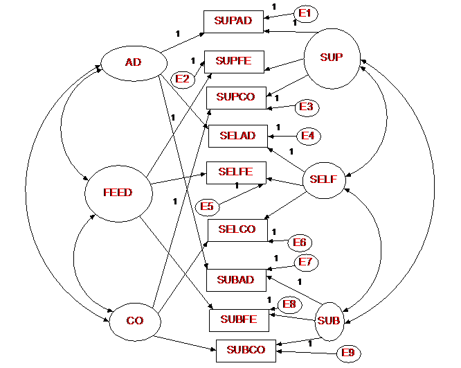
Standard CFA Estimation
The standard confirmatory factor analysis model of the MTMM is to have each
measure load on its trait and method factors. The traits factors are
correlated, as well as the method factors. Usually, the trait and
method factors are assumed to be independent. There must be at least
three traits and methods for this approach to be identified. The factor
loading structure is as follows:
Factor
Trait Method
Measures 1 2 3 1 2 3
T1M1 x x
T2M1 x x
T3M1 x x
T1M2 x x
T2M2 x x
T3M2 x x
T1M3 x x
T2M3 x x
T3M3 x x
where
an "x" means that the measure loads on the relevant trait or method
factor and no “x” implies a zero loading.
The
major advantage of Standard CFA MTMM approach with correlated errors is that
the variance of a measure can be orthogonally partitioned into trait, method,
and error variance.
Standard CFA
Identification Issues with Standard CFA Model
The standard model
requires at least a total 6 trait and method factors with at least 2 trait and
2 method factors. However, the standard
CFA model for the MTMM is not empirically identified for two very important
cases: when the loadings for each factor are exactly equal or when there
is no discriminant validity between two or more factors. Although actual data never exactly satisfy
these conditions, they usually approach one of the cases, and so the standard
CFA model is typically empirically
underidentified. Heywood
cases, impossible values (correlations larger than one and negative
variances), and convergence problems are quite commonly found during
estimation. Thus given these problems, the "standard" model can
be problematic. However, if there are
either a large number of traits or methods (5 or more), these estimation
problems may be alleviated.
Marsh and Bailey (1991) report that 77% time improper solutions result from the Standard CFA approach. Very often Heywood cases, there are Heywood cases. For instance for the example, five of the measures have non-significant error variances.
very strong correlations
uninterruptable results
example: a negative trait loading
failure to converge
wild estimates and huge standard errors
Even when this model appears to produce a good solution, trait variance tends to be "pushed" into method factors.
Source of the Problems
Empirical underidentification (despite the fact that fit is almost always excellent!)
Specialized submodels underidentified
Equal loadings, trait and methods factors uncorrelated (Wothke, 1984)
Equal loadings, traits and methods correlated (Kenny & Kashy, 1992)
Estimation dilemma
loadings equal: underidentification
loadings unequal: large loadings (Heywoods) and small loadings (empirical underidentification)
While these models have identification issues, it appears that models with a large (5 or more) number of traits, do not have such severe estimation problems.
For the Mount data the fit is quite good, χ²(12) = 9.19, p = .69. There are no Heywood cases, but several of the trait loadings are weak and one is negative.
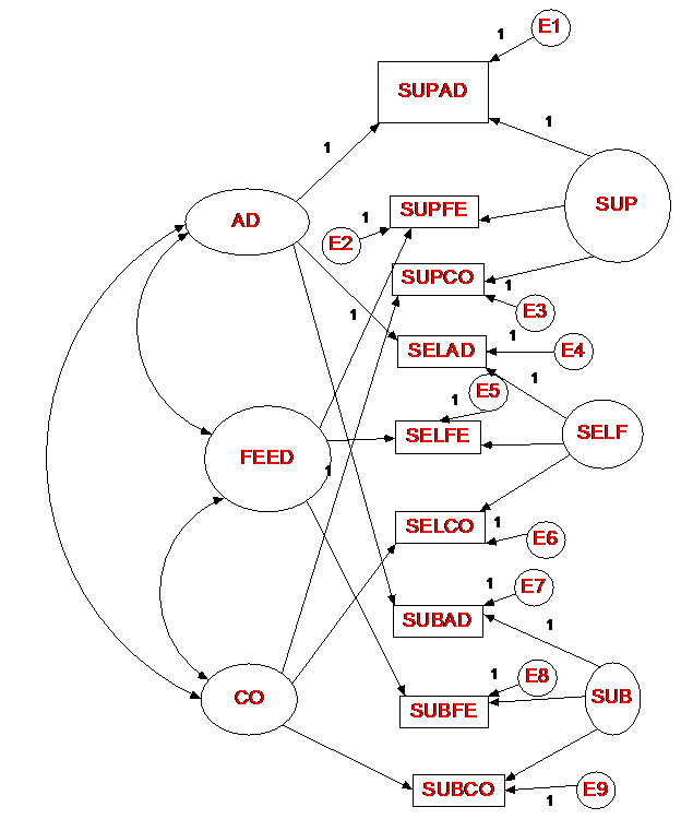
Standard CFA with
Uncorrelated Method Factors
This model is identical to the Standard CFA Model, but the method factors are
uncorrelated. Such a model has fewer
estimation problems than the Standard CFA Model. The
fit of the model is χ²(15) = 18.73, p =
.226. Here is the diagram:
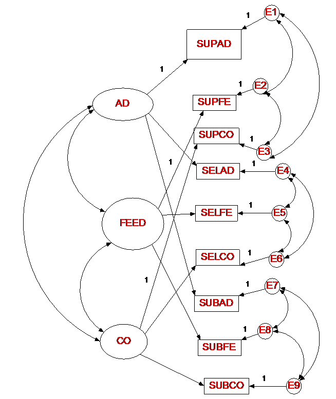
Correlated Uniqueness Model
In this model, there are no method factors, but measures that share a common
method have correlated errors or uniquenesses. The error
variance-covariance matrix would be as follows:
T1M1
x
T2M1
x x
T3M1
x x x
T1M2
x
T2M2
x x
T3M2
x x
x
T1M3
x
T2M3
x x
T3M3
x x x
T1M1 T2M1 T3M1 T1M2 T2M2 T3M2 T1M3 T2M3 T3M3
where
an "x" means that a free error variance or covariance and no “x”
implies a zero covariance.
For this model to be identified there must be at least two traits and three
methods. This model does not have the difficulties that the standard CFA
model has.
Represents traits (trait loadings & trait factor correlations) the same way as standard model and uncorrelated methods model. The difference is in how method variance is represented: There are no method factors. Instead, method variance is modeled using uniquenesses (what's left over in a measured variable after trait variance is accounted for). If there are method effects, the uniquenesses should be correlated.
Identification: at least two traits and three methods.
Advantages
Marsh & Bailey: proper solutions 98% of the time
almost always converges
usually interpretable results
Disadvantages
No real method factors and so method variance difficult to measure
Method does not allow for the decomposition of variance into trait, method and error like the prior two methods.
Strong assumptions
Trait-method and method-method correlations zero
Example
Good Fit: χ²(15) = 18.73, p = .226
Convergent Validity: size of the trait loadings
Admin Feedback Consid
Sup A .758
Sup F .385
Sup C .661
Self A .716
Self F .638
Self C .590
Sub A .441
Sub F .244
Sub C .579
convergent validity – average loading (assuming correlations are analyzed)
by trait: Admin (.638), Feedback (.422), and Consid (.610)
by method: Sup (.601), Self (.648), and Sub (.421)
discriminant validity
trait correlations; rAF = .475, rAC = .020, and rFC = .351.; good discriminant validity
method variance: average covariance of errors, ignoring sign (assuming correlations were inputted as data)
.177 Supervisor
.088 Self
.252 Subordinate
most method “variance” for the subordinate
Correlated Uniqueness
Multiplicative or Direct Product Model
Warning: This model in non-intuitive and difficult to follow.
This model was originally proposed by Campbell & O'Connell who found that method variance was not constant (same value added to every correlation), but rather was proportional to the different-method, different trait correlation.
The model assumes that the correlation between two variables is NOT an additive combination of trait effects and method effects (models described above assume that the correlation a function of the shared trait variance plus the shared method variance). The multiplicative model assumes that the correlation is a multiplicative function of trait similarity and method similarity. So, if two methods are completely dissimilar, the correlation the same trait measured by the two methods would be zero.
The correlation between two traits (D and F) with two methods (1 and 2) equals:
rD1,F2 = cD1cF2rDFr12
rD1,D2 = cD1cD2r12
rD1,F1 = cD1cF1rDF
cD1 -- the square root of the communality of measure D1 (the square root of one minus the error variance)
cF2 -- the square root of the communality of measure F2
rDF -- the correlation between traits D and F
r12 -- the overall similarity between methods 1 and 2
Interpretation
Variance decomposed into trait and error variance.
No measure of method variance. In fact, using a different method dilutes the true relationship between two latent variables, whereas for other MTMM approaches require different methods to obtain the “true” correlation.
One of the advantages of this method is
that it estimates a correlation matrix for the methods. With this matrix,
one can determine the similarity of the different methods. It is possible
that the similarity between methods might be one which would mean that the
methods that were nominally different were in fact the same. In essence,
the methods would have no discriminant validity.
There have been a few comparisons
between the empirical utility of the standard additive and this newer
multiplicative model. The additive model appears to work better.
Nonetheless, the multiplicative model deserves attention.
The method is not often used, perhaps for the following reasons:
1. Not intuitive. No proportions of trait and method variance, difficult to interpret.
2. Difficult to set up. You do not believe me? See below?
3. Studies have shown fairly frequent estimation problems.
4. Fit tends to be worse than for the additive models.
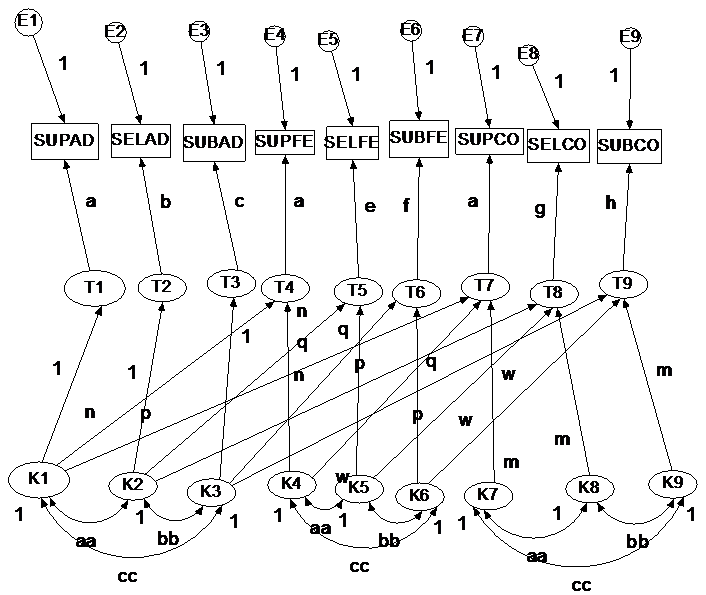
Estimation (not easy to follow; if you do not believe me strongly suggest looking at the figure below). Assume there are t traits and m methods. Initially order the measures from 1 to tm, such that method is fastest moving.
a. Each measure loads on its own factor, denoted as T from 1 to tm.
b. The loadings for first trait are all fixed to the same value (a in the figure below) and the other loadings are all free.
c. For each trait, create m standardized latent variables, denoted as K. As this done for each method there will be a total of tm such K factors.
d. Fix the correlations between the “same” K factors, i.e., between the same two methods, to be equal across traits.
e. Draw the following paths form the K to the T factors: For the first m K factor, fix the loadings to 1 for the first set, and then have them load on the other t – 1 sets, but fix the loadings to be the same. For the last set, just load on the last set. The K correlations will give the method correlations to establish method similarity.
f. When done flip the measures and traits such that traits are fastest moving. This will give the trait correlations that can be used to establish discriminant validity.
For the Mount example, the trait correlations are rAF = .451, rAC = .109, and rFC = .487 and the correlations between methods rSupSel = .510, rSupSub = .273, and rSelSub = .346. There are also three Heywood cases in the solution. In terms of model fit χ²(21) = 20.07, p = .96.
References
Campbell, D. T., & Fiske, D. W. (1959). Convergent and discriminant validation by the multitrait-multimethod matrix. Psychological Bulletin, 56, 81-105.
Campbell, D. T., & O'Connell, E. J. (1967). Method factors in multitrait-multimethod matrices: Multiplicative rather than additive? Multivariate Behavioral Research, 2, 409-426.
Kenny, D. A., & Kashy, D. A. (1992). Analysis of multitrait-multimethod matrix by confirmatory factor analysis. Psychological Bulletin, 112, 165-172.
Marsh,
H., & Bailey, M. (1991). Confirmatory factor analysis of
multitrait-multimethod data: A comparison of alternative models. Applied
Psychological Measurement, 15, 47-70.
Wothke, W. (1984). The estimation of trait and method components in multitrait multimethod measurement. Unpublished Doctoral Dissertation, University of Chicago.